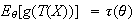
Appendix B: Statistics
The material in this appendix can be supplemented with the classic text in
statistics: The Theory of Point Estimation Wiley, New
York by E. Lehmann (1983).
Sufficiency, Completeness and Unbiased Estimation
In statistics, we often represent our data, in many cases a sample of size
 from some population as a random vector
 .
The model, can be written in the form
.
The model, can be written in the form
 where
where
 is the parameter space or set of permissible values of the parameter
and
is the parameter space or set of permissible values of the parameter
and
 is the probability density function. A statistic,
 is a function of the data which does not depend on the unknown parameter
 .
Although a statistic,
.
Although a statistic,
 is not a function of
 ,
its distribution can depend on
,
its distribution can depend on
 An estimator is a statistic considered for the purpose of estimating a given
parameter. One of our objectives is to find a ``good'' estimator of
the parameter
An estimator is a statistic considered for the purpose of estimating a given
parameter. One of our objectives is to find a ``good'' estimator of
the parameter
 ,
in some sense of the word ``good''. How do we ensure that a statistic
,
in some sense of the word ``good''. How do we ensure that a statistic
 is estimating the correct parameter and not consistently too large or too
small, and that as much variability as possible has been removed? The problem
of estimating the correct parameter is often dealt with by requiring that the
estimator be unbiased.
is estimating the correct parameter and not consistently too large or too
small, and that as much variability as possible has been removed? The problem
of estimating the correct parameter is often dealt with by requiring that the
estimator be unbiased.
We will denote an expected value under the assumed parameter value
 by
by
 .
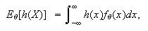
Thus, in the continuous case
.
Thus, in the continuous case
 and in the discrete case
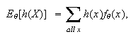 provided the integral/sum converges absolutely. In the discrete case,
 the probability function of
 under this parameter value

Definition
A statistic
 is an unbiased estimator of
 if
if
 for all
 .
.
For example suppose that
 are independent, each with the Poisson distribution with parameter
 .
Notice that the statistic
.
Notice that the statistic
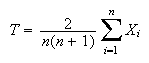 is such
that
is such
that and so
 is an unbiased estimator of
 This means that it is centered in the correct place, but does not mean it is a
best estimator in any sense.
This means that it is centered in the correct place, but does not mean it is a
best estimator in any sense.
In Decision Theory, in order to determine whether a given estimator
or statistic
 does well for estimating
 we consider a loss function or distance function between the estimator and the
true value. Call this
we consider a loss function or distance function between the estimator and the
true value. Call this
 .
Then this is averaged over all possible values of the data to obtain the risk:
.
Then this is averaged over all possible values of the data to obtain the risk:
 A good estimator is one with little risk, a bad estimator is one whose risk is
high. One particular risk function is called mean squared error
(M.S.E.) and corresponds to
A good estimator is one with little risk, a bad estimator is one whose risk is
high. One particular risk function is called mean squared error
(M.S.E.) and corresponds to
 .
The mean squared error has a useful decomposition into two components the
variance of the estimator and the square of its bias:
.
The mean squared error has a useful decomposition into two components the
variance of the estimator and the square of its bias:

For example, if
 has a
Normal
has a
Normal distribution, the mean squared error of
 is 1 for all
 because the bias
 is zero. On the other hand the estimator
 has bias
 and variance
 so the mean squared error is
 Obviously
 has smaller mean squared error provided that
 is
around 0 (more precisely provided
is
around 0 (more precisely provided
 ,
but for
,
but for
 large,
 is preferable. Of these two estimators, only
 is unbiased.
In general, in fact, there is usually no one estimator which outperforms all
other estimators at all values of the parameter if we use mean squared error
as our basis for comparison. In order to achieve an
optimal estimator, it is unfortunately necessary to restrict
ourselves to a specific class of estimators and select the best within the
class. Of course, the best within this class will only be as good as the class
itself (best in a class of one is not much of a recommendation), and therefore
we must ensure that restricting ourselves to this class is not unduly
restrictive. The class of all estimators is usually too large to
obtain a meaningful solution. One common restriction is to the class of all
unbiased estimators.
Definition
An estimator
 is said to be a uniformly minimum variance unbiased estimator
(U.M.V.U.E.) of the parameter
is said to be a uniformly minimum variance unbiased estimator
(U.M.V.U.E.) of the parameter
 if
if
(i) it is an unbiased estimator of
 and
and
(ii) among all unbiased estimators of
 it has the smallest mean squared error and therefore the smallest variance.
A sufficient statistic is one that, from a certain perspective,
contains all the necessary information for making inferences (e.g. estimating
the parameter with a point estimator or confidence interval, conducting a test
of a hypothesized value) about the unknown parameters in a given model. It is
important to remember that a statistic is sufficient for inference on a
specific parameter. It does not necessary contain all relevant information in
the data for other inferences. For example if you wished to test whether the
family of distributions is an adequate fit to the data ( a goodness of fit
test) the sufficient statistic for the parameter in the model does not contain
the relevant information.
Suppose the data is in a vector
 and
and
 is a sufficient statistic for
 .
The intuitive basis for sufficiency is that if the conditional distribution of
.
The intuitive basis for sufficiency is that if the conditional distribution of
 given
given
 does not depend on
 ,
then
,
then
 provides no additional value in addition to
 for estimating
 .
The assumption is that random variables carry information on a statistical
parameter
.
The assumption is that random variables carry information on a statistical
parameter
 only insofar as their distributions (or conditional distributions) change with
the value of the parameter and that since, given
only insofar as their distributions (or conditional distributions) change with
the value of the parameter and that since, given
 we can randomly generate at random values for the
 without knowledge of the parameter and with the correct distribution, these
randomly generated values cannot carry additional information. All of this, of
course, assumes that the model is correct and
without knowledge of the parameter and with the correct distribution, these
randomly generated values cannot carry additional information. All of this, of
course, assumes that the model is correct and
 is the only unknown. The distribution of
 given a sufficient statistic
 will often have value for other purposes, such as measuring the variability of
the estimator or testing the validity of the model.
will often have value for other purposes, such as measuring the variability of
the estimator or testing the validity of the model.
Definition
A statistic
 is sufficient for a statistical model
 if the distribution of the data
 given
given
 does not depend on the unknown parameter
 .
.
The use of a sufficient statistic is formalized in the The
Sufficiency Principle, which states that if
 is a sufficient statistic for a model

 and
and

 are two different possible observations that have identical values of the
sufficient statistic:
are two different possible observations that have identical values of the
sufficient statistic:
 then whatever inference we would draw from observing
 we should draw exactly the same inference from
 .
.
Sufficient statistics are not unique. For example if the
sample mean
 is a sufficient statistic, then any other statistic, that allows us to obtain
 is also sufficient. This will include all one-to-one functions of
 (these are essentially equivalent) like
 and all statistics
 for which we can write
 for some, possibly many-to-one function
 .
One result which is normally used to verify whether a given statistic is
sufficient is the Factorization Criterion for Sufficiency:
Suppose
.
One result which is normally used to verify whether a given statistic is
sufficient is the Factorization Criterion for Sufficiency:
Suppose
 has probability density function
 and
and
 is a statistic. Then
 is a sufficient statistic for
 if and only if there exist two non--negative functions
 and
and
 so that we can factor the probability density function
 for all
 This factorization into two pieces, one which involves both the statistic
 and the unknown parameter
 and the other which may be a constant or depend on
 but does not depend on the unknown parameter, need only hold on a set
 of possible values of
 which carries the full probability. That is for some set
 with
with
 for all
 ,
we require
,
we require
Definition
A statistic
 is a minimal sufficient statistic for
 if it is sufficient and if for any other sufficient statistic
 ,
there exists a function
,
there exists a function
 such that
 .
.
This definition says in effect that a minimal sufficient statistic can be
recovered from any other sufficient statistic. A statistic
 implicitly partitions the sample space into events of the form
![$[T(X)=x]$](graphics/appendixb__114.png) for varying
for varying
 and if
 is minimal sufficient, it induces the coarsest possible partition (i.e. the
largest possible sets) in the sample space among all sufficient statistics.
This partition is called the minimal sufficient partition.
is minimal sufficient, it induces the coarsest possible partition (i.e. the
largest possible sets) in the sample space among all sufficient statistics.
This partition is called the minimal sufficient partition.
The property of completeness is one which is useful for determining
the uniqueness of estimators and verifying in some cases that a minimal
sufficient reduction has been found. It bears no relation to the notion of a
complete market in Finance, or the mathematical notion of a complete metric
space. Let
 denote the observations from a distribution with probability density function
 .
Suppose
.
Suppose
 is a statistic and
 ,
a function of
,
a function of
 ,
is an unbiased estimator of
,
is an unbiased estimator of
 so that


 .
Under what circumstances is this the only unbiased estimator which is a
function of
.
Under what circumstances is this the only unbiased estimator which is a
function of
 ?
To answer this question, suppose
?
To answer this question, suppose
 and
and
 are both unbiased estimators of
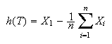
 and consider the difference
 .
Since
.
Since
 and
and
 are both unbiased estimators of the parameter
 we have
![$E_{\theta}[h(T)]=0$](graphics/appendixb__135.png) for all
for all
 .
Now if the only function
.
Now if the only function
 which satisfies
![$E_{\theta}[h(T)]=0$](graphics/appendixb__138.png) for all
for all
 is the zero function
 ,
then the two unbiased estimators must be identical. A statistic
,
then the two unbiased estimators must be identical. A statistic
 with this property is said to be complete. Technically it is not the
statistic that is complete, but the family of distributions of
with this property is said to be complete. Technically it is not the
statistic that is complete, but the family of distributions of
 in the model
Definition
The statistic
 is complete if
 for any function
 implies
For example, let
 be a random sample from the
Normal
be a random sample from the
Normal distribution. Consider
 .
Then
.
Then
 is sufficient for
 but is not complete. It is easy to see that it is not complete, because the
function
but is not complete. It is easy to see that it is not complete, because the
function
 is a function of
 which has zero expectation for all values of
 and yet the function is not identically zero. The fact that the statistic
 is sufficient but not complete is a hint that further reduction is possible,
that it is not minimal sufficient. In fact in this case, as we will show a
little later, taking only the second component of
is sufficient but not complete is a hint that further reduction is possible,
that it is not minimal sufficient. In fact in this case, as we will show a
little later, taking only the second component of
 namely
 provides a minimal sufficient, complete statistic.
Theorem B1
If
 is a complete and sufficient statistic for the model
 ,
then
,
then
 is a minimal sufficient statistic for the model.
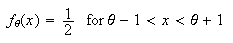
The converse to the above theorem is not true. Let
 be a random sample from the continuous uniform distribution on the interval
 .
This distribution has probability density function
.
This distribution has probability density function
 Then using the factorization criterion above, the joint probability density
function for a sample of
Then using the factorization criterion above, the joint probability density
function for a sample of
 independent observations from this density is
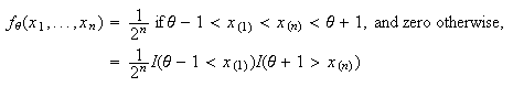 where
where
 is one or zero as the inequality holds or does not hold and
 are the smallest and the largest values in the sample
 Obviously
 can be written as a function
 where
where
 and so
 is sufficient. Moreover it is not difficult to show that no further reduction
(for example to
is sufficient. Moreover it is not difficult to show that no further reduction
(for example to
 alone) is possible or we can not longer provide such a factorization, so
 us minimal sufficient. Nevertheless, if
 and the function
 is defined by
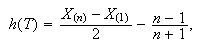 (clearly a non-zero function) then
![$E_{\theta}[h(T)]=0$](graphics/appendixb__179.png) for all
for all
 and therefore
 is not a complete statistic.
Theorem B2
For any random variables
 and
and
 ,
,
 and
and
In much of what follows, we wish to be able to estimate a general
function of the unknown parameter like
 instead of the parameter
 itself. We have already seen that if
 is a complete statistic, then there is at most one function of
 that provides an unbiased estimator of any function of a given
 In fact if we can find such a function,
 then it automatically has minimum variance among all possible unbiased
estimators of
then it automatically has minimum variance among all possible unbiased
estimators of
 that are based on the same data.
Theorem B3
If
 is a complete sufficient statistic for the model
 and
and
 ,
then
,
then
 is the U.M.V.U.E. of
 .
.
When we have a complete sufficient statistic, and we are able to find an
unbiased estimator, even a bad one, of
 then there is a simple recipe for determining the U.M.V.U.E. of

Theorem B4
If
 is a complete sufficient statistic for the model
 and
and
 is any unbiased estimator of
 ,
then
,
then
 is the U.M.V.U.E. of
 .
.
Note that we did not subscript the conditional expectation
 with
with
 because whenever
 is a sufficient statistic, the conditional distribution of
 given
given
 does not depend on the underlying value of the parameter

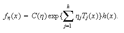
Definition
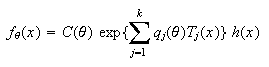
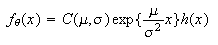
Suppose
 has a (joint) probability density function of the form
 for functions


 .
Then we say that the density is a member of the exponential family of
densities. We call
.
Then we say that the density is a member of the exponential family of
densities. We call
 the natural sufficient statistic.
A member of the exponential family could be re-expressed in different ways and
so the natural sufficient statistic is not unique. For example we may multiply
a given
 by a constant and divide the corresponding
 by the same constant, resulting in the same probability density function
 .
Various other conditions need to be applied as well, for example to insure
that the
.
Various other conditions need to be applied as well, for example to insure
that the
 are all essentially different functions of the data. One of the important
properties of the exponential family is its closure under repeated independent
sampling. In general if
are all essentially different functions of the data. One of the important
properties of the exponential family is its closure under repeated independent
sampling. In general if
 are independent identically distributed with an exponential family
distribution then their joint distribution
are independent identically distributed with an exponential family
distribution then their joint distribution
 is also an exponential family distribution.
Theorem B5
Let
( be a random sample from the distribution with probability density function
given by (exfd). Then
be a random sample from the distribution with probability density function
given by (exfd). Then
 also has an exponential family form, with joint probability density function
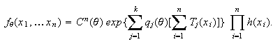
In other words,
 is replaced by
 and
and
 by
by
 .
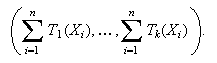
The natural sufficient statistic is
.
The natural sufficient statistic is
It is usual to reparameterize equation
(exfd) by replacing
 by a new parameter
 .
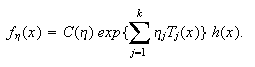
This results in a more efficient representation, the canonical form
of the exponential family density:
.
This results in a more efficient representation, the canonical form
of the exponential family density:
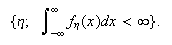
 The natural parameter space in this form is the set of all values of
 for which the above function is integrable; that is
 We would like this parameter space to be large enough to allow intervals for
each of the components of the vector
We would like this parameter space to be large enough to allow intervals for
each of the components of the vector
 and so we will later need to assume that the natural parameter space contains
a
and so we will later need to assume that the natural parameter space contains
a
 dimensional
rectangle.
dimensional
rectangle.
If the statistic satisfies a linear constraint, for example,
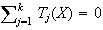 with probability one, then the number of terms
 could be reduced and a more efficient representation of the probability
density function is possible. Similarly if the parameters
could be reduced and a more efficient representation of the probability
density function is possible. Similarly if the parameters
 satisfy a linear relationship, they are not all statistically meaningful
because one of the parameters is obtainable from the others. These are all
situations that we would handle by reducing the model to a more efficient and
non-redundant form. So in the remaining, we will generally assume such a
reduction has already been made and that the exponential family representation
is minimal in the sense that neither the
satisfy a linear relationship, they are not all statistically meaningful
because one of the parameters is obtainable from the others. These are all
situations that we would handle by reducing the model to a more efficient and
non-redundant form. So in the remaining, we will generally assume such a
reduction has already been made and that the exponential family representation
is minimal in the sense that neither the
 nor the
 satisfy any linear constraints.
Definition
We will say that
 has a regular exponential family distribution if it is in canonical
form, is of full rank in the sense that neither the
has a regular exponential family distribution if it is in canonical
form, is of full rank in the sense that neither the
 nor the
 satisfy any linear constraints permitting a reduction in the value of
 ,
and the natural parameter space contains a
,
and the natural parameter space contains a
 dimensional
rectangle.
dimensional
rectangle.
By Theorem B5, if
 has a regular exponential family distribution then
 also has a regular exponential family distribution.
The main advantage identifying a distribution as a member of the regular
exponential family is that it allows to to quickly identify the minimal
sufficient statistic and conclude that it is complete.
Theorem B6
If
 has a regular exponential family distribution then
 is a complete sufficient statistic.
Example
Let
 be independent observations all from the normal
 distribution. Notice that with the parameter
 we can write the probability density function of each
 as a constant

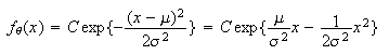 so the natural parameters are
 and
and
 and the natural sufficient statistic is
(
and the natural sufficient statistic is
( For a sample of size
 from this density we have the same natural parameters, and, by the above
theorem, a complete sufficient statistic is
(
from this density we have the same natural parameters, and, by the above
theorem, a complete sufficient statistic is
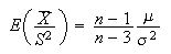
( For example if you wished to find a U.M.V.U.E. of any function of
 , for example the parameter
 we need only find some function of the compete sufficient statistic which has
the correct expected value. For example, in this case, with the sample mean
we need only find some function of the compete sufficient statistic which has
the correct expected value. For example, in this case, with the sample mean
 and the sample variance
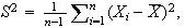 it is not difficult to show that
 and so, provided

 is an unbiased estimator and a function of the complete sufficient statistic
so it is the desired U.M.V.U.E. Suppose one of the parameters, say
is an unbiased estimator and a function of the complete sufficient statistic
so it is the desired U.M.V.U.E. Suppose one of the parameters, say
 is assumed known. Then the normal distribution is still in the regular
exponential family, since it has a representation
is assumed known. Then the normal distribution is still in the regular
exponential family, since it has a representation
 with the function
 completely known. In this case, for a sample of size
 from this distribution, the statistic
 is complete sufficient for
 and so any function of it, say
 which is an unbiased estimator of
 is automatically U.M.V.U.E.
The Table below gives various members of the regular exponential family and
the corresponding complete sufficient statistic.
| Members of the Regular Exponential Family |
|
Complete Sufficient Statistic |
 |
|
 |
 |
|
 |
 Binomial
 |
|
 |
Geometric( |
|
 |
 |
if
 known
known |
 |
 |
 known
known |
 |
 |
|
 |
 (includes exponential)
 |
if
 known
known |
 |
 |
if
 known
known |
 |
 |
|
 |
Differentiating under the Integral
For a regular exponential family, it is possible to differentiate under the
integral, that is,
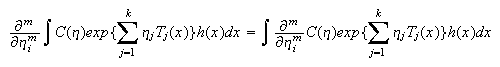 for any
 and any
 in the interior of the natural parameter space.
Let
 denote observations from a distribution with probability density function
 and let
 be a statistic. The information on the parameter
 is provided by the sensitivity of the distribution of a statistic to changes
in the parameter. For example, suppose a modest change in the parameter value
leads to a large change in the expected value of the distribution resulting in
a large shift in the data. Then the parameter can be estimated fairly
precisely. On the other hand, if a statistic
is provided by the sensitivity of the distribution of a statistic to changes
in the parameter. For example, suppose a modest change in the parameter value
leads to a large change in the expected value of the distribution resulting in
a large shift in the data. Then the parameter can be estimated fairly
precisely. On the other hand, if a statistic
 has no sensitivity at all in distribution to the parameter, then it would
appear to contain little information for point estimation of this parameter. A
statistic of the second kind is called an ancillary statistic.
has no sensitivity at all in distribution to the parameter, then it would
appear to contain little information for point estimation of this parameter. A
statistic of the second kind is called an ancillary statistic.
Definition
 is an ancillary statistic if its distribution does not depend on the
unknown parameter
is an ancillary statistic if its distribution does not depend on the
unknown parameter
 .
.
Ancillary statistics are, in a sense, orthogonal or perpendicular to minimal
sufficient statistics and are analogous to the residuals in a multiple
regression, while the complete sufficient statistics are analogous to the
estimators of the regression coefficients. It is well-known that the residuals
are uncorrelated with the estimators of the regression coefficients (and
independent in the case of normal errors). However, the ``irrelevance'' of the
ancillary statistic seems to be limited to the case when it is not part of the
minimal (preferably complete) sufficient statistic as the following example
illustrates.
Example
Suppose a fair coin is tossed to determine a random variable
 with probability
 and
and
 otherwise. We then observe a Binomial random variable
 with parameters
 .
Then the minimal sufficient statistic is
.
Then the minimal sufficient statistic is
 but
but
 is an ancillary statistic since its distribution does not depend on the
unknown parameter
is an ancillary statistic since its distribution does not depend on the
unknown parameter
 .
Is
.
Is
 completely irrelevant to inference about
 ?
If you reported to your boss an estimator of
?
If you reported to your boss an estimator of
 such as
 without telling him or her the value of
 how long would you expect to keep your job? Clearly any sensible inference
about
how long would you expect to keep your job? Clearly any sensible inference
about
 should include information about the precision of the estimator, and this
inevitably requires knowing the value of
should include information about the precision of the estimator, and this
inevitably requires knowing the value of
 Although the distribution of
 does not depend on the unknown parameter
 so that
 is ancillary, it carries important information about precision. The following
theorem allows us to use the properties of completeness and ancillarity to
prove the independence of two statistics without finding their joint
distribution.
is ancillary, it carries important information about precision. The following
theorem allows us to use the properties of completeness and ancillarity to
prove the independence of two statistics without finding their joint
distribution.
Basu's Theorem B7
Consider
 with probability density function
 .
Let
.
Let
 be a complete sufficient statistic. Then
 is independent of every ancillary statistic
 .
.
Example
Assume
 represents the market price of a given asset such as a portfolio of stocks at
time
represents the market price of a given asset such as a portfolio of stocks at
time
 and
and
 is the value of the portfolio at the beginning of a given time period (assume
that the analysis is conditional on
is the value of the portfolio at the beginning of a given time period (assume
that the analysis is conditional on
 so that
 is fixed and known). The process
 is assumed to be a Brownian motion and so the distribution of
 for any fixed time
 is
Normal
is
Normal for
for
 .
Suppose that for a period of length 1, we record both the period high
.
Suppose that for a period of length 1, we record both the period high
 and the close
 .
Define random variables
.
Define random variables
 and
and
 .
Then the joint probability density function of
.
Then the joint probability density function of
 can be shown to be
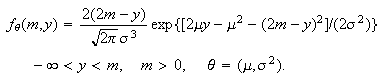
It is not hard to show that this is a member of the regular exponential family
of distributions with both parameters assumed unknown. If one parameter is
known, for example,
 ,
it is again a regular exponential family distribution with
,
it is again a regular exponential family distribution with
 Consequently, if we record independent pairs of observations

 on the portfolio for a total of
 distinct time periods (and if we assume no change in the parameters), then the
statistic
distinct time periods (and if we assume no change in the parameters), then the
statistic
 is a complete sufficient statistic for the drift parameter
 .
Since it is also an unbiased estimator of
.
Since it is also an unbiased estimator of
 it is the U.M.V.U.E. of
 .
By Basu's theorem it will be independent of any ancillary statistic, i.e. any
statistic whose distribution does not depend on the parameter
.
By Basu's theorem it will be independent of any ancillary statistic, i.e. any
statistic whose distribution does not depend on the parameter
 One such statistic is
 which is therefore independent of

Maximum Likelihood Estimation
Suppose we have observed
 independent discrete random variables all with probability density function
 where the scalar parameter
 is unknown. Suppose our observations are
 .
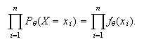
Then the probability of the observed data is:
.
Then the probability of the observed data is:
 When the observations have been substituted, this becomes a function of the
parameter only, referred to as the likelihood function and denoted
When the observations have been substituted, this becomes a function of the
parameter only, referred to as the likelihood function and denoted
 .
Its natural logarithm is usually denoted
.
Its natural logarithm is usually denoted
 .
Now in the absence of any other information, it seems logical that we should
estimate the parameter
.
Now in the absence of any other information, it seems logical that we should
estimate the parameter
 using a value most compatible with the data. For example we might choose the
value maximizing the likelihood function
using a value most compatible with the data. For example we might choose the
value maximizing the likelihood function
 or equivalently maximizing
 .
We call such a maximizer the maximum likelihood (M.L.) estimate
provided it exists and satisfies any restrictions placed on the parameter. We
denote it by
.
We call such a maximizer the maximum likelihood (M.L.) estimate
provided it exists and satisfies any restrictions placed on the parameter. We
denote it by
 .
Obviously, it is a function of the data, that is,
.
Obviously, it is a function of the data, that is,
 .
The corresponding estimator is
.
The corresponding estimator is
 .
In practice we are usually satisfied with a local maximum of the
likelihood function provided that it is reasonable, partly because the global
maximization problem is often quite difficult, partly because the global
maximum is not always better than a local maximum near a preliminary estimator
that is known to be consistent.. In the case of a twice differentiable log
likelihood function on an open interval, this local maximum is usually found
by solving the equation
.
In practice we are usually satisfied with a local maximum of the
likelihood function provided that it is reasonable, partly because the global
maximization problem is often quite difficult, partly because the global
maximum is not always better than a local maximum near a preliminary estimator
that is known to be consistent.. In the case of a twice differentiable log
likelihood function on an open interval, this local maximum is usually found
by solving the equation
 for a solution
 ,
where
,
where
 is called the score function. The equation
 is called the (maximum) likelihood equation or score equation. To
verify a local maximum we compute the second derivative
is called the (maximum) likelihood equation or score equation. To
verify a local maximum we compute the second derivative
 and show that it is negative, or alternatively show
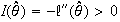 .
The function
.
The function
 is called the information function. In a sense to be investigated
later,
is called the information function. In a sense to be investigated
later,
 ,
the observed information, indicates how much information about a
parameter is available in a given experiment. The larger the value, the more
curved is the log likelihood function and the easier it is to find the
maximum.
,
the observed information, indicates how much information about a
parameter is available in a given experiment. The larger the value, the more
curved is the log likelihood function and the easier it is to find the
maximum.
Although we view the likelihood, log likelihood, score and information
functions as functions of
 they are, of course, also functions of the observed data
 .
When it is important to emphasize the dependence on the data
.
When it is important to emphasize the dependence on the data
 we will write

 etc. Also when we wish to determine the sampling properties of these functions
as functions of the random variable
etc. Also when we wish to determine the sampling properties of these functions
as functions of the random variable
 we will write

 etc.
etc.
Definition
The Fisher or expected information (function) is the expected value
of the information function
 .
.
Likelihoods for Continuous Models
Suppose a random variable
 has a continuous probability density function
 with parameter
 .
We will often observe only the value of
.
We will often observe only the value of
 rounded to some degree of precision (say 1 decimal place) in which case the
actual observation is a discrete random variable. For example, suppose we
observe
rounded to some degree of precision (say 1 decimal place) in which case the
actual observation is a discrete random variable. For example, suppose we
observe
 correct to one decimal place. Then
 assuming the function
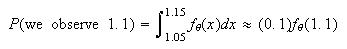
 is quite smooth over the interval. More generally, if we observe
 rounded to the nearest
 (assumed small) then the likelihood of the observation is approximately
 .
Since the precision
.
Since the precision
 of the observation does not depend on the parameter, then maximizing the
discrete likelihood of the observation is essentially equivalent to maximizing
the the probability density function
of the observation does not depend on the parameter, then maximizing the
discrete likelihood of the observation is essentially equivalent to maximizing
the the probability density function
 over the parameter. This partially justifies the use of the probability
density function in the continuous case as the likelihood function.
over the parameter. This partially justifies the use of the probability
density function in the continuous case as the likelihood function.
Similarly, if we observed
 independent values
 of a continuous random variable, we would maximize the likelihood
 (or more commonly its logarithm) to obtain the maximum likelihood estimator of
 .
.
The relative likelihood function
 defined as
 is the ratio of the likelihood to its maximum value and takes on values
between
is the ratio of the likelihood to its maximum value and takes on values
between
 and
and
 .
It is used to rank possible parameter values according to their plausibility
in light of the data. If
.
It is used to rank possible parameter values according to their plausibility
in light of the data. If
 ,
say, then
,
say, then
 is rather an implausible parameter value because the data are ten times more
likely when
is rather an implausible parameter value because the data are ten times more
likely when
 than they are when
 .
The set of
.
The set of
 -values
for which
-values
for which
 is called a
 likelihood region for
 When
the parameter
When
the parameter
 is one-dimensional, and
 is its true value,
 converges in distribution as the sample size
 to a chi-squared distribution with 1 degree of freedom. More generally, the
numbers of degrees of freedom of the limiting chi-squared distribution is the
dimension of the parameter
to a chi-squared distribution with 1 degree of freedom. More generally, the
numbers of degrees of freedom of the limiting chi-squared distribution is the
dimension of the parameter
 We can use this to construct a confidence interval for the unknown value of
the parameter. For example if
We can use this to construct a confidence interval for the unknown value of
the parameter. For example if
 is chosen to be the 0.95 quantile of the chi-squared(1) distribution
(
is chosen to be the 0.95 quantile of the chi-squared(1) distribution
( ,
then
,
then
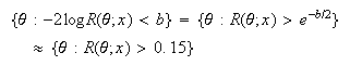 so a
so a
 likelihood interval is an approximate
 confidence interval for
 .
This seems to indicate that the confidence interval tolerates a considerable
difference in the likelihood. The likelihood at a parameter value must differ
from the maximum likelihood by a factor of more than
.
This seems to indicate that the confidence interval tolerates a considerable
difference in the likelihood. The likelihood at a parameter value must differ
from the maximum likelihood by a factor of more than
 before it is excluded by a
 confidence interval or rejected by a test with level of significance 5%.
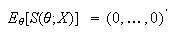
Properties of the Score and Information
Consider a continuous model with a family of probability density functions
 .
Suppose all of the densities are supported on a common set
.
Suppose all of the densities are supported on a common set
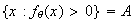 .
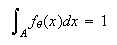
Then
.
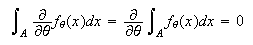
Then
 and therefore
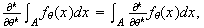
 provided that the integral can be interchanged with the derivative. Models
that permit this interchange, and calculation of the Fisher information, are
called regular models.
provided that the integral can be interchanged with the derivative. Models
that permit this interchange, and calculation of the Fisher information, are
called regular models.
Regular Models
Consider a statistical model
 with each density supported by a common set
 .
Suppose
.
Suppose
 is an open interval in the real line and
 for all
 and
and
 .
Suppose in addition
.
Suppose in addition
-
![$\ln[f_{\theta}(x)]$](graphics/appendixb__447.png) is a continuous, three times differentiable function of
is a continuous, three times differentiable function of
 for all
 .
.
-

-
 for some function
 satisfying
 .
.
-
 .
.
Then we call this a regular family of distributions or a regular
model. Similarly, if these conditions hold with
 a discrete random variable and the integrals replaced by sums, the family is
also called regular. Conditions like these permitting the interchange
of expected values and derivative are sometimes referred to as the Cramer
conditions. In general, they are used to justify passage of a derivative under
an integral.
a discrete random variable and the integrals replaced by sums, the family is
also called regular. Conditions like these permitting the interchange
of expected values and derivative are sometimes referred to as the Cramer
conditions. In general, they are used to justify passage of a derivative under
an integral.
Theorem B8
If
 is a random sample from a regular model
 then
then
 and
and

The Multiparameter Case
The case of several parameters is exactly analogous to the scalar parameter
case. Suppose
 .
In this case the ``parameter'' can be thought of as a column vector of
.
In this case the ``parameter'' can be thought of as a column vector of
 scalar parameters. The score function
 is a
is a
 dimensional
column vector whose
dimensional
column vector whose
 component is the derivative of
 with respect to the
 component of
 ,
that is,
,
that is,
 The observed information function
 is a
is a
 matrix whose
 element is

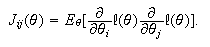
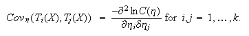
 The Fisher information is a
 matrix whose components are component-wise expectations of the information
matrix, that is
matrix whose components are component-wise expectations of the information
matrix, that is
 The definition of a regular family of distributions is similarly extended. For
a regular family of distributions
The definition of a regular family of distributions is similarly extended. For
a regular family of distributions
 and the covariance matrix of the score function
var
and the covariance matrix of the score function
var is the Fisher information, i.e.
Maximum likelihood Estimation in the Exponential Family
Suppose
 has a regular exponential family distribution of the form
 Then
Then
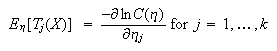 and
and
 Therefore the maximum likelihood estimator of
 based on a random sample
 from
from
 is the solution to the
 equations
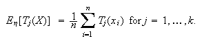 The maximum likelihood estimators are obtained by setting the sample moments
of the natural sufficient statistic equal to their expected values and
solving.
The maximum likelihood estimators are obtained by setting the sample moments
of the natural sufficient statistic equal to their expected values and
solving.
Finding Maximum likelihood estimates using Newton's Method
Suppose that the maximum likelihood estimate
 is determined by the likelihood equation
 It frequently happens that an analytic solution for
 cannot be obtained. If we begin with an approximate value for the parameter,
 ,
we may update that value as follows:
,
we may update that value as follows:
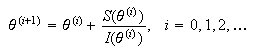 and provided that convergence of

 obtains, it converges to a solution to the score equation above. In the
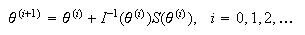
multiparameter case, where
obtains, it converges to a solution to the score equation above. In the
multiparameter case, where
 is a vector and
 is a matrix, then Newton's method becomes:
 In both of these, we can replace the information function by the Fisher
information for a similar
algorithm.
In both of these, we can replace the information function by the Fisher
information for a similar
algorithm.
Suppose we consider estimating a parameter
 where
where
 is a scalar, using an unbiased estimator
 .
Is there any limit to how well an estimator like this can behave? The answer
for unbiased estimators is in the affirmative. A lower bound on the variance
is given by the information inequality.
.
Is there any limit to how well an estimator like this can behave? The answer
for unbiased estimators is in the affirmative. A lower bound on the variance
is given by the information inequality.
Information Inequality
Suppose
 is an unbiased estimator of the parameter
 in a regular statistical model
 .
Then
.
Then
 Equality holds if and only if
 is regular exponential family with natural sufficient statistic
 .
.
If equality holds in (CRLB) then we call
 an efficient estimator of
 .
The number on the right hand side of (CRLB),
.
The number on the right hand side of (CRLB),

-
is called the Cramér-Rao lower bound (C.R.L.B.).
We often express the efficiency of an unbiased
estimator using the ratio of (C.R.L.B.) to the variance of the estimator.
Large values of the efficiciency (i.e. near one) indicate that the variance of
the estimator is close to the lower bound.
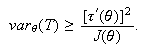
The special case of the information inequality that is of most interest is the
unbiased estimation of the parameter
 .
The above inequality indicates that any unbiased estimator
.
The above inequality indicates that any unbiased estimator
 of
of
 has variance at least
 .
The lower bound is achieved only when
.
The lower bound is achieved only when
 is regular exponential family with natural sufficient statistic
 ,
so even in the exponential family, only certain parameters are such that we
can find unbiased estimators which achieve the C.R.L.B., namely those that are
expressible as the expected value of the natural sufficient statistics.
,
so even in the exponential family, only certain parameters are such that we
can find unbiased estimators which achieve the C.R.L.B., namely those that are
expressible as the expected value of the natural sufficient statistics.
The Multiparameter Case
The right hand side in the information inequality generalizes naturally to the
multiple parameter case in which
 is a vector. For example if
 ,
then the Fisher information
,
then the Fisher information
 is a
is a
 matrix. If
 is any real-valued function of
 then its derivative is a column
vector
then its derivative is a column
vector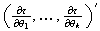 .
Then if
.
Then if
 is any unbiased estimator of
 in a regular model,
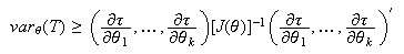 for all
 .
.
Asymptotic Properties of maximum likelihood Estimators
One of the more successful attempts at justifying estimators and demonstrating
some form of optimality has been through large sample theory or the
asymptotic behaviour of estimators as the sample size
 .
One of the first properties one requires is consistency of an estimator. This
means that the estimator converges to the true value of the parameter as the
sample size (and hence the information) approaches infinity.
.
One of the first properties one requires is consistency of an estimator. This
means that the estimator converges to the true value of the parameter as the
sample size (and hence the information) approaches infinity.
Definition
Consider a sequence of estimators
 where the subscript
 indicates that the estimator has been obtained from data
 with sample size
 .
Then the sequence is said to be a consistent sequence of estimators
of
.
Then the sequence is said to be a consistent sequence of estimators
of
 if
if
 for all
 .
.
It is worth a reminder at this point that probability density functions are
used to produce probabilities and are only unique up to a point. For example
if two probability density functions
 and
and
 were such that they produced the same probabilities, or the same cumulative
distribution function, for example,
were such that they produced the same probabilities, or the same cumulative
distribution function, for example,
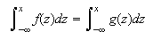 for all
 then we would not consider them distinct probability densities, even though
 and
and
 may differ at one or more values of
 .
Now when we parameterize a given statistical model using
.
Now when we parameterize a given statistical model using
 as the parameter, it is natural to do so in such a way that different
values of the parameter lead to distinct probability density functions.
This means, for example, that the cumulative distribution functions associated
with these densities are distinct. Without this assumption, made in the
following theorem, it would be impossible to accurately estimate the parameter
since two different parameters could lead to the same cumulative distribution
function and hence exactly the same behaviour of the observations.
as the parameter, it is natural to do so in such a way that different
values of the parameter lead to distinct probability density functions.
This means, for example, that the cumulative distribution functions associated
with these densities are distinct. Without this assumption, made in the
following theorem, it would be impossible to accurately estimate the parameter
since two different parameters could lead to the same cumulative distribution
function and hence exactly the same behaviour of the observations.
Theorem B9
Suppose
 is a random sample from a regular statistical model
{
is a random sample from a regular statistical model
{ .
Assume the densities corresponding to different values of the parameters are
distinct. Let
.
Assume the densities corresponding to different values of the parameters are
distinct. Let


 .
Then with probability tending to
.
Then with probability tending to
 as
as
 ,
the likelihood equation
,
the likelihood equation
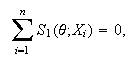 has a root
 such that
 converges in probability to
 ,
the true value of the parameter, as
,
the true value of the parameter, as
 .
.
The likelihood equation above does not always have a unique root. The
consistency of the maximum likelihood estimator is one indication that it
performs reasonably well. However, it provides no reason to prefer it to some
other consistent estimator. The following result indicates that maximum
likelihood estimators perform as well as any reasonable estimator can, at
least in the limit as
 .
Most of the proofs of these asymptotic results can be found in Lehmann(1991).
.
Most of the proofs of these asymptotic results can be found in Lehmann(1991).
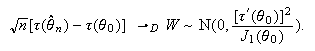
Theorem B10
Suppose
 is a random sample from a regular statistical model

 .
Suppose
.
Suppose
 is a consistent root of the likelihood equation as in the theorem above. Let
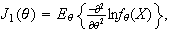 the Fisher information for a sample of size one. Then
 where
where
 is the true value of the parameter.
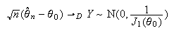
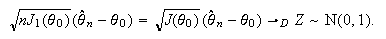
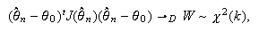
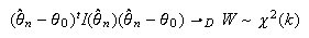
This result may also be written as
This theorem asserts that, at least under the regularity required, the maximum
likelihood estimator is asymptotically unbiased. Moreover, the asymptotic
variance of the maximum likelihood estimator approaches the Cramér-Rao
lower bound for unbiased estimators. This justifies the comparison of the
variance of an estimator
 based on a sample of size
 to the value
 ,
which is the asymptotic variance of the maximum likelihood estimator
and also the Cramér-Rao lower bound.
,
which is the asymptotic variance of the maximum likelihood estimator
and also the Cramér-Rao lower bound.
It also follows that
 This indicates that the asymptotic variance of any function
 of the maximum likelihood estimator also achieves the Cramér-Rao lower
bound.
of the maximum likelihood estimator also achieves the Cramér-Rao lower
bound.
Definition
Suppose
 is asymptotically normal with mean
 and variance
 .
The asymptotic efficiency of
.
The asymptotic efficiency of
 is defined to be
 .
This is the ratio of the Cramér-Rao lower bound to the variance of
.
This is the ratio of the Cramér-Rao lower bound to the variance of
 and is typically less than one, close to one indicating the asymptotic
efficiency is close to that of the maximum likelihood estimator.
and is typically less than one, close to one indicating the asymptotic
efficiency is close to that of the maximum likelihood estimator.
The Multiparameter Case
In the case
 ,
the score function is the vector of partial derivatives of the log likelihood
with respect to the components of
,
the score function is the vector of partial derivatives of the log likelihood
with respect to the components of
 .
Therefore the likelihood equation is
.
Therefore the likelihood equation is
 equations in the
 unknown parameters. Under similar regularity conditions to the univariate
case, the conclusion of Theorem B9 holds in this case, that is, the components
of
unknown parameters. Under similar regularity conditions to the univariate
case, the conclusion of Theorem B9 holds in this case, that is, the components
of
 each converge in probability to the corresponding component of
 .
Similarly, the asymptotic normality remains valid in this case with little
modification. Let
.
Similarly, the asymptotic normality remains valid in this case with little
modification. Let
 be the Fisher information matrix for a sample of size one and assume it is a
non-singular matrix. Then
be the Fisher information matrix for a sample of size one and assume it is a
non-singular matrix. Then
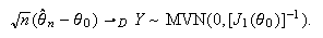 where
the multivariate normal distribution with
where
the multivariate normal distribution with
 -dimensional
mean vector
-dimensional
mean vector
 and covariance matrix
 (
( )
, denoted
)
, denoted
 has probability density function defined on
 ,
,
It also follows that
 where
where
 .
Once again the asymptotic variance-covariance matrix is identical to the lower
bound given by the multiparameter case of the Information Inequality.
.
Once again the asymptotic variance-covariance matrix is identical to the lower
bound given by the multiparameter case of the Information Inequality.
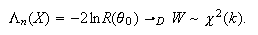
Joint confidence regions can be constructed based on one of the asymptotic
results

 or
or
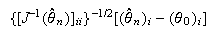
 Confidence intervals for a single parameter, say
 ,
can be based on the approximate normality of
,
can be based on the approximate normality of
 or
or
 where
where
 is the
 entry in the vector
 and
and
![$[A^{-1}]_{ii}$](graphics/appendixb__603.png) is the
is the
 entry in the matrix
 .
.
Unidentifiability and Singular Information Matrices
Suppose we observe two independent random variables
 having normal distributions with the same variance
 and means

 respectively. In this case, although the means depend on the parameter
 ,
the value of this vector parameter is unidentifiable in the sense
that, for some pairs of distinct parameter values, the probability density
function of the observations are identical. For example the parameter
,
the value of this vector parameter is unidentifiable in the sense
that, for some pairs of distinct parameter values, the probability density
function of the observations are identical. For example the parameter
 leads to exactly the same joint distribution of
 as does the parameter
 .
In this case, we we might consider only the two parameters
.
In this case, we we might consider only the two parameters
 and anything derivable from this pair estimable, while parameters such as
 that cannot be obtained as functions of
 are consequently unidentifiable. The solution to the original identifiability
problem is the reparametrization to the new parameter
are consequently unidentifiable. The solution to the original identifiability
problem is the reparametrization to the new parameter
 in this case, and in general, unidentifiability usually means one should seek
a new, more parsimonious parametrization.
in this case, and in general, unidentifiability usually means one should seek
a new, more parsimonious parametrization.
In the above example, compute the Fisher information matrix for the parameter
 .
Notice that the Fisher information matrix is singular. This means that if you
were to attempt to compute the asymptotic variance of the maximum likelihood
estimator of
.
Notice that the Fisher information matrix is singular. This means that if you
were to attempt to compute the asymptotic variance of the maximum likelihood
estimator of
 by inverting the Fisher information matrix, the inversion would be impossible.
Attempting to invert a singular matrix is like attempting to invert the number
0. It results in one or more components that you can consider to be infinite.
Arguing intuitively, the asymptotic variance of the maximum likelihood
estimator of some of the parameters is infinite. This is an indication that
asymptotically, at least, some of the parameters may not be identifiable. When
parameters are unidentifiable, the Fisher information matrix is generally
singular. However, when
by inverting the Fisher information matrix, the inversion would be impossible.
Attempting to invert a singular matrix is like attempting to invert the number
0. It results in one or more components that you can consider to be infinite.
Arguing intuitively, the asymptotic variance of the maximum likelihood
estimator of some of the parameters is infinite. This is an indication that
asymptotically, at least, some of the parameters may not be identifiable. When
parameters are unidentifiable, the Fisher information matrix is generally
singular. However, when
 is singular for all values of
 ,
this may or may not mean parameters are unidentifiable for finite sample
sizes, but it does usually mean one should take a careful look at the
parameters with a possible view to adopting another parametrization.
,
this may or may not mean parameters are unidentifiable for finite sample
sizes, but it does usually mean one should take a careful look at the
parameters with a possible view to adopting another parametrization.
U.M.V.U.E.'s and maximum likelihood
Estimators: A Comparison
Which of the two main types of estimators should we use? There is no general
consensus among statisticians.
-
If we are estimating the expectation of a natural sufficient statistic
 in a regular exponential family both maximum likelihood and unbiasedness
considerations lead to the use of
in a regular exponential family both maximum likelihood and unbiasedness
considerations lead to the use of
 as an estimator.
-
When sample sizes are large U.M.V.U.E's and maximum likelihood estimators are
essentially the same. In that case use is governed by ease of computation.
Unfortunately how large ``large'' needs to be is usually unknown. Some studies
have been carried out comparing the behaviour of U.M.V.U.E.'s and maximum
likelihood estimators for various small fixed sample sizes. The results are,
as might be expected, inconclusive.
-
maximum likelihood estimators exist ``more frequently'' and when they do they
are usually easier to compute than U.M.V.U.E.'s. This is essentially because
of the appealing invariance property of maximum likelihood estimators.
-
Simple examples are known for which maximum likelihood estimators behave badly
even for large samples. This is more often the case when there is a large
number of parameters, some of which, termed ``nuisance parameters'' are of no
direct interest, but complicate the estimation.
-
U.M.V.U.E.'s and maximum likelihood estimators are not necessarily robust. A
small change in the underlying distribution or the data could result in a
large change in the estimator.
Other Estimation Criteria
Best Linear Unbiased Estimators
The problem of finding best unbiased estimators is considerably simpler if we
limit the class in which we search. If we permit any function of the data,
then we usually require the heavy machinery of complete sufficiency to produce
U.M.V.U.E.'s. However, the situation is much simpler if we suggest some
initial random variables and then require that our estimator be a linear
combination of these. Suppose, for example we have random variables
 with
with

 where
where
 is the parameter of interest and
 is another parameter. What linear combinations of the
 's
provide an unbiased estimator of
's
provide an unbiased estimator of
 and among these possible linear combinations which one has the smallest
possible variance? To answer these questions, we need to know the covariances
and among these possible linear combinations which one has the smallest
possible variance? To answer these questions, we need to know the covariances
 (at least up to some scalar multiple). Suppose
 and
var
and
var .
Let
.
Let
 and
and
 We can write the model in a form reminiscent of linear regression as
 where
where
 and the
 's
are uncorrelated random variables with
's
are uncorrelated random variables with
 and
var
and
var .
Then the linear combination of the components of
.
Then the linear combination of the components of
 that has the smallest variance among all unbiased estimators of
 is given by the usual regression formula
 and
and
 provides the best estimator of
 in the sense of smallest variance. In other words, the linear combination of
the components of
in the sense of smallest variance. In other words, the linear combination of
the components of
 which has smallest variance among all unbiased estimators of
 is
is
 where
where
 .
In the above example, we may compute the Fisher information matrix for the
parameter
.
In the above example, we may compute the Fisher information matrix for the
parameter
 as follows.
The log likelihood is
 and
the Fisher information is the covariance matrix of the score vector
and
the Fisher information is the covariance matrix of the score vector
 and
this is
and
this is
 Notice
that
Notice
that
 is, in this case, singular. If you were to attempt to compute the asymptotic
variance of the maximum likleihood estimator of
is, in this case, singular. If you were to attempt to compute the asymptotic
variance of the maximum likleihood estimator of
 by inverting this information matrix, the inversion is impossible. Attempting
to invert a singular matrix is like attempting the inverse of
by inverting this information matrix, the inversion is impossible. Attempting
to invert a singular matrix is like attempting the inverse of
 , one or more components of the inverse can be taken to be infinite,
indicating that, asymptotically at least, one of more of the parameters is
unidentifiable.
, one or more components of the inverse can be taken to be infinite,
indicating that, asymptotically at least, one of more of the parameters is
unidentifiable.
More generally, we wish to consider a number
 of possibly dependent random variables
 whose expectations may be related to a parameter
 .
These may, for example, be individual observations or a number of competing
estimators constructed from these observations. We assume
.
These may, for example, be individual observations or a number of competing
estimators constructed from these observations. We assume
 has expectation given by
 where
where
 is some
 matrix having rank
 and
and
 is a vector of unknown parameters. As in multiple regression, the matrix
 is known and non-random. Suppose the covariance matrix of
 is
is
 with
with
 a known non-singular matrix and
 a possibly unknown scalar parameter. We wish to estimate a linear combination
of the components of
a possibly unknown scalar parameter. We wish to estimate a linear combination
of the components of
 ,
say
,
say
 where
where
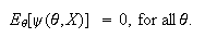 is a known
 -dimensional
column vector. We restrict our attention to unbiased estimators of
-dimensional
column vector. We restrict our attention to unbiased estimators of
 .
.
Gauss-Markov Theorem B11
Theorem B11: Gauss-Markov Theorem
Suppose
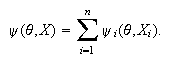 is a random vector with mean and covariance matrix
 where
matrices
where
matrices
 and
and
 are known and the parameters
 and
and
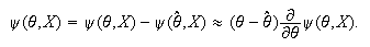 unknown. Suppose we wish to estimate a linear combination
 of the components of
 .
Then among all linear combinations of the components of
.
Then among all linear combinations of the components of
 which are unbiased estimators of the parameter
 the estimator
 has
the smallest variance.
has
the smallest variance.
Note that this result does not depend on any assumed normality of the
components of
 but only on the first and second moment behaviour, that is, the mean and the
covariances. The special case when
but only on the first and second moment behaviour, that is, the mean and the
covariances. The special case when
 is the identity matrix is the least squares estimator.
Estimating Equations
To find the maximum likelihood estimator, we usually solve the likelihood
equation
 Note that the function on the left hand side is a function of both the
observations and the parameter. Such a function is called an estimating
function. Most sensible estimators, like the maximum likelihood
estimator, can be described easily through an estimating function. For
example, if we know
var
Note that the function on the left hand side is a function of both the
observations and the parameter. Such a function is called an estimating
function. Most sensible estimators, like the maximum likelihood
estimator, can be described easily through an estimating function. For
example, if we know
var for independent identically distributed
 ,
then we can use the estimating function
,
then we can use the estimating function
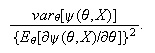 to estimate the parameter
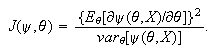 ,
without any other knowledge of the distribution, its density, mean etc. The
estimating function is set equal to 0 and solved for
,
without any other knowledge of the distribution, its density, mean etc. The
estimating function is set equal to 0 and solved for
 .
The above estimating function is an unbiased estimating function in
the sense that
.
The above estimating function is an unbiased estimating function in
the sense that
 This allows us to conclude that the function is at least centered
appropriately for the estimation of the parameter
This allows us to conclude that the function is at least centered
appropriately for the estimation of the parameter
 .
Now suppose that
.
Now suppose that
 is an unbiased estimating function corresponding to a large sample. Often it
can be written as the sum of independent components, for example
is an unbiased estimating function corresponding to a large sample. Often it
can be written as the sum of independent components, for example
 Now suppose
 is a root of the estimating equation
 Then for
 sufficiently close to
 ,
,
 Uusing the Central Limit Theorem, assuming that
 is the true value of the parameter and provided
 is a sum as in (B3.5), the left hand side of
(ef2) is approximately normal with mean
is a sum as in (B3.5), the left hand side of
(ef2) is approximately normal with mean
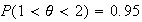 and variance equal to
var
and variance equal to
var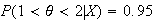 .
The term
.
The term
 is also a sum of similar derivatives of the individual
 .
If a law of large numbers applies to these terms, then when divided by
.
If a law of large numbers applies to these terms, then when divided by
 this sum will be asymptotically equivalent to
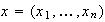 .
It follows that the root
.
It follows that the root
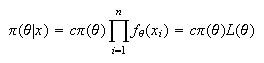 will have an approximate normal distribution with mean
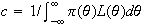 and variance
 By analogy with the relation between asymptotic variance of the maximum
likelihood estimator and the Fisher information, we call the reciprocal of the
above asymptotic variance formula the Godambe information of the
estimating function. This information measure is
By analogy with the relation between asymptotic variance of the maximum
likelihood estimator and the Fisher information, we call the reciprocal of the
above asymptotic variance formula the Godambe information of the
estimating function. This information measure is
 Godambe(1960) proved the following result.
Theorem B12
Among all unbiased estimating functions satisfying the usual regularity
conditions, an estimating function which maximizes the Godambe information
(B3.6) is of the form
 where
where
 is non-random.
Bayesian Methods
There are two major schools of thought on the way in which statistical
inference is conducted, the frequentist and the Bayesian
school. Typically, these schools differ slightly on the actual
methodology and the conclusions that are reached, but more substantially on
the philosophy underlying the treatment of parameters. So far we have
considered a parameter as an unknown constant underlying or indexing the
probability density function of the data. It is only the data, and statistics
derived from the data that are random.
The Bayesian begins with the assertion that the parameter
 obtains as the realization of some larger random experiment. The parameter is
assumed to have been generated according to some distribution, the prior
distribution
obtains as the realization of some larger random experiment. The parameter is
assumed to have been generated according to some distribution, the prior
distribution
 and the observations then obtained from the corresponding probability density
function
and the observations then obtained from the corresponding probability density
function
 interpreted as the conditional probability density of the data given the value
of
interpreted as the conditional probability density of the data given the value
of
 .
The prior distribution
.
The prior distribution
 quantifies information about
 prior to any further data being gathered. Sometimes
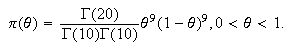 can be constructed on the basis of past data. For example, if a quality
inspection program has been running for some time, the distribution of the
number of defectives in past batches can be used as the prior distribution for
the number of defectives in a future batch. The prior can also be chosen to
incorporate subjective information based on an expert's experience and
personal judgement. The purpose of the data is then to adjust this
distribution for
can be constructed on the basis of past data. For example, if a quality
inspection program has been running for some time, the distribution of the
number of defectives in past batches can be used as the prior distribution for
the number of defectives in a future batch. The prior can also be chosen to
incorporate subjective information based on an expert's experience and
personal judgement. The purpose of the data is then to adjust this
distribution for
 in the light of the data, to result in the posterior distribution for
the parameter. Any conclusions about the plausible value of the parameter are
to be drawn from the posterior distribution. For a frequentist, statements
like
in the light of the data, to result in the posterior distribution for
the parameter. Any conclusions about the plausible value of the parameter are
to be drawn from the posterior distribution. For a frequentist, statements
like
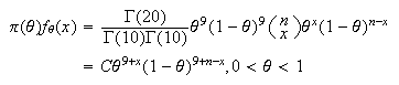 are meaningless; all randomness lies in the data and the parameter is an
unknown constant. Frequentists are careful to assure students that if an
observed 95% confidence interval for the parameter is
are meaningless; all randomness lies in the data and the parameter is an
unknown constant. Frequentists are careful to assure students that if an
observed 95% confidence interval for the parameter is
 this does not imply
 .
However, a Bayesian will happily quote such a probability, usually
conditionally on some observations, for example,
.
However, a Bayesian will happily quote such a probability, usually
conditionally on some observations, for example,
 .
In spite of some distance in the philosophy regarding the (random?) nature of
statistical parameters, the two paradigms tend to largely agree for large
sample sizes because the prior assumptions of the Bayesian tend to be a small
contributor to the conclusion.
.
In spite of some distance in the philosophy regarding the (random?) nature of
statistical parameters, the two paradigms tend to largely agree for large
sample sizes because the prior assumptions of the Bayesian tend to be a small
contributor to the conclusion.
Posterior Distributions
Suppose the parameter is initially chosen at random according to the prior
distribution
 and then given the value of the parameter the observations are
independent identically distributed, each with conditional probability
(density) function
and then given the value of the parameter the observations are
independent identically distributed, each with conditional probability
(density) function
 .
Then the posterior distribution of the parameter is the conditional
distribution of
.
Then the posterior distribution of the parameter is the conditional
distribution of
 given the data

 where
where
 is independent of
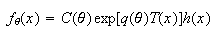 and
and
 is the likelihood function. Since Bayesian inference is based on the posterior
distribution it depends only on the data through the likelihood function.
is the likelihood function. Since Bayesian inference is based on the posterior
distribution it depends only on the data through the likelihood function.
Example
Suppose a coin is tossed
 times with probability of heads
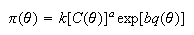 .
It is known from my ``very considerable previous experience with coins'' that
the prior probability of heads is not always identically
.
It is known from my ``very considerable previous experience with coins'' that
the prior probability of heads is not always identically
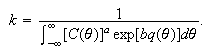 but follows a
BETA
but follows a
BETA distribution. If the
 tosses result in
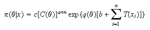 heads, we wish to find the posterior density function for
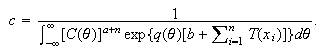 .
In this case the prior distribution for the parameter
.
In this case the prior distribution for the parameter
 is the Beta(10,10) distribution with probability density function
 The posterior distribution of
 is therefore proportional to
 where the constant
 may depend on
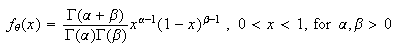 but dos not depend on
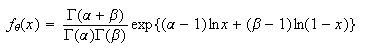 Therefore the posterior distribution is also a Beta distribution but with
parameters
Therefore the posterior distribution is also a Beta distribution but with
parameters
 Notice that the posterior mean is the expected value of this beta distribution
and is
Notice that the posterior mean is the expected value of this beta distribution
and is
 which, for
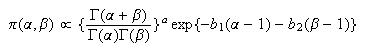 and
and
 sufficiently large, is reasonably close to the usual estimator

Conjugate Prior Distributions
If a prior distribution has the property that the posterior distribution is in
the same family of distributions as the prior then the prior is called a
conjugate prior.
Suppose
 is a random sample from the exponential family
 and
and
 is assumed to have the prior distribution with parameters
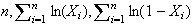 given by
 where
where
 Then the posterior distribution of
 ,
given the data
,
given the data
 is easily seen to be given by
 where
where
 Notice that the posterior distribution is in the same family of distributions
as (3.8) and thus
Notice that the posterior distribution is in the same family of distributions
as (3.8) and thus
 is a conjugate prior. The value of the parameters of the posterior
distribution reflect the choice of parameters in the prior.
is a conjugate prior. The value of the parameters of the posterior
distribution reflect the choice of parameters in the prior.
Example
To find the conjugate prior for
 (
( for a random sample
 from the
beta(
from the
beta( distribution with probability density function
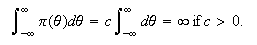 we begin by writing this in exponential family
form,
we begin by writing this in exponential family
form, Then the conjugate prior distribution is the joint probability density
function
Then the conjugate prior distribution is the joint probability density
function
 on
(
on
( which is proportional to
 for parameters
 The posterior distribution takes the same form as
(priorbeta) but with the parameters
The posterior distribution takes the same form as
(priorbeta) but with the parameters
 replaced by
 Bayesians are sometimes criticised for allowing their subjective opinions (in
this case leading to the choice of the prior parameters
Bayesians are sometimes criticised for allowing their subjective opinions (in
this case leading to the choice of the prior parameters
 influence the resulting inference but notice that in this case, and more
generally, as the sample size
influence the resulting inference but notice that in this case, and more
generally, as the sample size
 grows, the value of the parameters of the posterior distribution is mostly
determined by the components
grows, the value of the parameters of the posterior distribution is mostly
determined by the components
 above which grow in
 eventually washing out the influence of the choice of prior parameters.
Noninformative Prior Distributions
The choice of the prior distribution to be the conjugate prior is often
motivated by mathematical convenience. However, a Bayesian would also like the
prior to accurately represent the preliminary uncertainty about the plausible
values of the parameter, and this may not be easily translated into one of the
conjugate prior distributions. Noninformative priors are the usual way of
representing ignorance about
 and they are frequently used in practice. It can be argued that they are more
objective than a subjectively assessed prior distribution since the latter may
contain personal bias as well as background knowledge. Also, in some
applications the amount of prior information available is far less than the
information contained in the data. In this case there seems little point in
worrying about a precise specification of the prior distribution.
and they are frequently used in practice. It can be argued that they are more
objective than a subjectively assessed prior distribution since the latter may
contain personal bias as well as background knowledge. Also, in some
applications the amount of prior information available is far less than the
information contained in the data. In this case there seems little point in
worrying about a precise specification of the prior distribution.
In the coin tossing example above, we assumed a Beta(10,10) prior distribution
for the probability of heads. If were no reason to prefer one value of
 over any other then a noninformative or `flat' prior disribution for
 that could be used is the
UNIF
that could be used is the
UNIF distribution, also as it turns out a special case of the beta distribution.
Ignorance may not be bliss but for Bayesians it is most often uniformly
distributed. For estimating the mean
distribution, also as it turns out a special case of the beta distribution.
Ignorance may not be bliss but for Bayesians it is most often uniformly
distributed. For estimating the mean
 of a
N
of a
N distribution the possible values for
 are
are
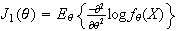 .
If we take the prior distribution to be uniform on
.
If we take the prior distribution to be uniform on
 ,
that is,
,
that is,
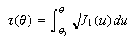 then this is not a proper probability density since
 Prior densities of this type are called improper priors. In this case we could
consider a sequence of prior distributions such as the
UNIF
Prior densities of this type are called improper priors. In this case we could
consider a sequence of prior distributions such as the
UNIF which approximates this prior as
 .
Suppose we call such a prior density function
.
Suppose we call such a prior density function
 .
Then the posterior distribution of the parameter is given by
.
Then the posterior distribution of the parameter is given by
 and it is easy to see that as
 ,
this approaches a constant multiple of the likelihood function
,
this approaches a constant multiple of the likelihood function
 .
For reasonably large sample size,
.
For reasonably large sample size,
 is often integrable and can therefore be normalized to produce a proper
posterior distribution, even though the corresponding prior was improper. This
Bayesian development provides an alternate interpretation of the likelihood
function. We can consider it as proportional to the posterior distribution of
the parameter when using a uniform improper prior on the whole real
line. The language is somewhat sloppy here since, as we have seen, the uniform
distribution on the whole real line really makes sense only through taking
limits for uniform distributions on finite intervals.
is often integrable and can therefore be normalized to produce a proper
posterior distribution, even though the corresponding prior was improper. This
Bayesian development provides an alternate interpretation of the likelihood
function. We can consider it as proportional to the posterior distribution of
the parameter when using a uniform improper prior on the whole real
line. The language is somewhat sloppy here since, as we have seen, the uniform
distribution on the whole real line really makes sense only through taking
limits for uniform distributions on finite intervals.
In the case of a scale parameter, which must take positive values such as the
normal variance, it is usual to express ignorance of the prior distribution of
the parameter by assuming that the logarithm of the parameter is uniform on
the real line.
One possible difficulty with using nonformative prior distributions is the
concern whether the prior distribution should be uniform for
 itself or some function of
 ,
such as
,
such as
 or
or
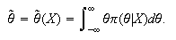 The objective when we used a uniform prior for a probability was to add no
more information about the parameter around one possible value than around
some other, and so it makes sense to use a uniform prior for a parameter that
essentially has uniform information attached to it. For this reason, it is
common to use a uniform prior for
The objective when we used a uniform prior for a probability was to add no
more information about the parameter around one possible value than around
some other, and so it makes sense to use a uniform prior for a parameter that
essentially has uniform information attached to it. For this reason, it is
common to use a uniform prior for
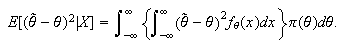 where
where
 is the function of
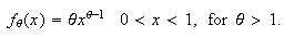 whose Fisher information,
 is constant. This idea is due to Jeffreys and leads to a prior distribution
which is proportional to
is constant. This idea is due to Jeffreys and leads to a prior distribution
which is proportional to
![$[J(\theta)]^{1/2}.$](graphics/appendixb__813.png) Such a prior is referred to as a Jeffreys' prior. The
reparametrization which leads to a Jeffrey's prior can be carried out as
follows: suppose
Such a prior is referred to as a Jeffreys' prior. The
reparametrization which leads to a Jeffrey's prior can be carried out as
follows: suppose
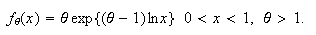
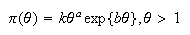 is a regular model and
 is the Fisher information for a single observation. Then if we choose an
abitrary value for
is the Fisher information for a single observation. Then if we choose an
abitrary value for
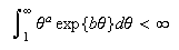 and define the reparameterization
 Then in this case, the Fisher information for the parameter
 ,
,
 equals one for all values of
 and so Jeffry's prior corresponds to using a uniform prior distribution on the
values of
and so Jeffry's prior corresponds to using a uniform prior distribution on the
values of
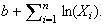 Since the asymptotic variance of the maximum likelihood estimator
 is
equal to
is
equal to
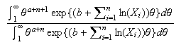 ,
which does not depend on
,
which does not depend on
 (3.9)
is often called a variance stabilizing transformation.
(3.9)
is often called a variance stabilizing transformation.
Bayes Point Estimators
One method of obtaining a point estimator of
 is to use the posterior distribution and a suitable loss function.
Theorem B13
The Bayes estimator of
 for
squared error loss with respect to the prior
for
squared error loss with respect to the prior
 given data
 is the mean of the posterior distribution given by
 This estimator minimizes

Example
Suppose
 is a random sample from the distribution with probability density function
 Using a conjugate prior for
 find the Bayes estimator of
 for squared error loss.
We begin by identifying the conjugate prior distribution. Since
 the conjugate prior density is
 which is evidently a Gamma distribution restricted to the interval
 and if the prior is to be proper, the parameters must be chosen such that
 so
so
 Then the posterior distribution takes the same form as the prior but with
 replaced by
 and
and
 by
by
 The Bayes estimate of
 for squared error loss is the mean of this posterior distribution, or

Bayesian Interval estimates
There remains, after many decades, a controversy between Bayesians and
frequentists about which approach to estimation is more suitable to the real
world. The Bayesian has advantages at least in the ease of interpretation of
the results. For example, a Bayesian can use the posterior distribution given
the data
 to determine points

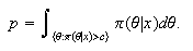 such that
 and then give a Bayesian confidence interval
 for the parameter. If this results in the interval
 the Bayesian will state that (in a Bayesian model, subject to the validity of
the prior) the conditional probability given the data that the parameter falls
in the interval
the Bayesian will state that (in a Bayesian model, subject to the validity of
the prior) the conditional probability given the data that the parameter falls
in the interval
 is
is
 .
No such probability can be ascribed to a confidence interval for frequentists,
who see no randomness in the parameter to which this probability statement is
supposed to apply. Bayesian confidence regions are also called credible
regions in order to make clear the distinction between the interpretation
of Bayesian confidence regions and frequentist confidence regions.
.
No such probability can be ascribed to a confidence interval for frequentists,
who see no randomness in the parameter to which this probability statement is
supposed to apply. Bayesian confidence regions are also called credible
regions in order to make clear the distinction between the interpretation
of Bayesian confidence regions and frequentist confidence regions.
Suppose
 is the posterior distribution of
 given the data
 and
and
 is a subset of
 .
If
.
If
 then
then
 is called a
 credible region for
 A credible region can be formed in many ways. If
 is an interval such that
 then
then
 is called a
 equal-tailed credible region. A highest posterior density (H.P.D.)
credible region is constructed in a manner similar to likelihood regions. The
equal-tailed credible region. A highest posterior density (H.P.D.)
credible region is constructed in a manner similar to likelihood regions. The
 highest posterior density. credible region is given by
 where
where
 is chosen such that
 A highest posterior density credible region is optimal in the sense that it is
the shortest
A highest posterior density credible region is optimal in the sense that it is
the shortest
 credible interval for a given value of
 .
.
Example
Suppose
 is a random sample from the
N
is a random sample from the
N distribution where
 is known and
 has the conjugate prior. Find the
 H.P.D. credible region for
 .
Compare this to a
.
Compare this to a
 C.I. for

Suppose the prior distribution for
 is
is
 so the prior density is given by
 and
the posterior density by
and
the posterior density by
 where
the constants
where
the constants
 and
and
 depend on
 but not on
 and where
 Therefore
the posterior distribution of
Therefore
the posterior distribution of
 is
is
 It follows that the 0.95 H.P.D. credible region is of the form
 Notice
that as
Notice
that as
 the weight
 and so
 is asymptotically equivalent to the sample mean
 Similarly, as

 is asymptotically equivalent to
 .
This means that for large values of
.
This means that for large values of
 the H.P.D. region is close to the region
 and
the latter is the 95% confidence interval for
and
the latter is the 95% confidence interval for
 based on the normal distribution of the maximum likelihood estimator

Finally, although statisticians argue whether the Bayesian or the frequentist
approach is better, there is really no one right way to do statistics. There
is something fundamentalist about the Bayesian paradigm, (though the Reverand
Bayes was, as far as we know, far from a fundamentalist) in that it places all
objects, parameters and data, in much the same context and treats them
similarly. It is a coherent philosophy of statistics, and a Bayesian will
vigorously argue that there is an inconsistency in regarding some unknowns as
random and others deterministic. There are certainly instances in which a
Bayesian approach seems more sensible-- particularly for example if the
parameter is a measurement on a possibly randomly chosen individual (say the
expected total annual claim of a client of an insurance company).
Hypothesis Tests
Statistical estimation usually concerns the estimation of the value of a
parameter when we know little about it except perhaps that it lies in a given
parameter space, and when we have no a priori reason to prefer one
value of the parameter over another. If, however, we are asked to decide
between two possible values of the parameter, the consequences of one choice
of the parameter value may be quite different from another choice. For
example, if we believe
 is normally distributed with mean
 and variance
 for some explanatory variables
 ,
then the value
,
then the value
 means there is no relation between
 and
and
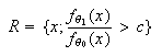 .
We need neither collect the values of
.
We need neither collect the values of
 nor build a model around them. Thus the two choices
 and
and
 are quite different in their consequences. This is often the case.
A hypothesis test involves a (usually natural) separation of the parameter
space
 into two disjoint regions,
 and
and
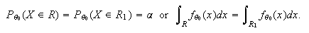 .
By the difference between the two sets we mean those points in the former
.
By the difference between the two sets we mean those points in the former
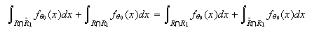 that are not in the latter
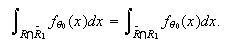 .
This partition of the parameter space corresponds to testing the null
hypothesis that the parameter is in
.
This partition of the parameter space corresponds to testing the null
hypothesis that the parameter is in
 .
We usually write this hypothesis in the form
.
We usually write this hypothesis in the form
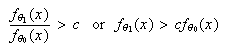 The null hypothesis is usually the status quo. For example in a test of a new
drug, the null hypothesis would be that the drug had no effect, or no more of
an effect than drugs already on the market. The null hypothesis is only
rejected if there is reasonably strong evidence against it. The
alternative hypothesis determines what departures from the null
hypothesis are anticipated. In this case, it might be simply
The null hypothesis is usually the status quo. For example in a test of a new
drug, the null hypothesis would be that the drug had no effect, or no more of
an effect than drugs already on the market. The null hypothesis is only
rejected if there is reasonably strong evidence against it. The
alternative hypothesis determines what departures from the null
hypothesis are anticipated. In this case, it might be simply
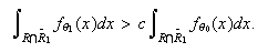 Since we do not know the true value of the parameter, we must base our
decision on the observed value of
Since we do not know the true value of the parameter, we must base our
decision on the observed value of
 .
The hypothesis test is conducted by determining a partition of the
sample space into two sets, the critical or rejection region
.
The hypothesis test is conducted by determining a partition of the
sample space into two sets, the critical or rejection region
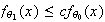 and its complement
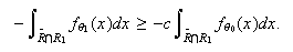 which is called the acceptance region. We declare that
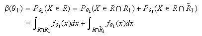 is false (in favour of the alternative) if we observe
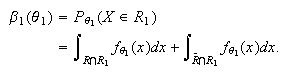 .
.
Definition
The power function of a test with critical region
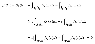 is the function
 or the probability that the null hypothesis is rejected as a function of the
parameter.
or the probability that the null hypothesis is rejected as a function of the
parameter.
It is obviously desirable, in order to minimize the two types of possible
errors in our decision, for the power function
 to be small for
 but large otherwise. The probability of rejecting the null hypothesis when it
is true (type I error) is a particularly important type of error
which we attempt to minimize. This probability determines one important
measure of the performance of a test, the level of significance.
but large otherwise. The probability of rejecting the null hypothesis when it
is true (type I error) is a particularly important type of error
which we attempt to minimize. This probability determines one important
measure of the performance of a test, the level of significance.
Definition
A test has level of significance
 if
if
 for all
 .
.
The level of significance is simply an upper bound on the probability of a
type I error. There is no assurance that the upper bound is tight, that is,
that equality is achieved somewhere. The lowest such upper bound is often
called the size of the test.
Definition
The size of a test is equal to
 .
.
Uniformly Most Powerful Tests
Tests are often constructed by specifying the size of the test, which in turn
determines the probability of the type I error, and then attempting to
minimize the probability that the null hypothesis is accepted when it is false
(type II error). Equivalently, we try and maximize the power function
of the test for
 .
.
Definition
A test with power function
 is a uniformly most powerful (U.M.P.) test of size
 if, for all other tests of the same size
 having power function
 ,
we have
,
we have
 for all
 .
.
The word ``uniformly'' above refers to the fact that one function dominates
another, that is,
 uniformly for all
 .
When the alternative
.
When the alternative
 consists of a single point
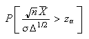 then the construction of a best test is particularly easy. In this case, we
may drop the word ``uniformly'' and refer to a ``most powerful test''. The
construction of a best test, by this definition, is possible under rather
special circumstances. First, we often require a simple null
hypothesis. This is the case when
then the construction of a best test is particularly easy. In this case, we
may drop the word ``uniformly'' and refer to a ``most powerful test''. The
construction of a best test, by this definition, is possible under rather
special circumstances. First, we often require a simple null
hypothesis. This is the case when
 consists of a single point
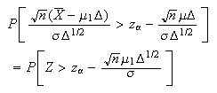 and so we are testing the null hypothesis
 .
.
Neyman-Pearson Lemma B14
Let
 have probability (density) function
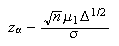
 .
Consider testing a simple null hypothesis
.
Consider testing a simple null hypothesis
 against a simple alternative
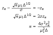 .
For a constant
.
For a constant
 ,
suppose the critical region defined by
,
suppose the critical region defined by
 corresponds to a test of size
 .
Then the test with this critical region is a most powerful test of size
.
Then the test with this critical region is a most powerful test of size
 for testing
 against
 .
.
Proof:
Consider another critical region
 with the same size. Then
 Therefore
 and
and
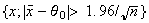
For
 ,
,
 and thus
 For
For

 ,
and thus
,
and thus
Now
 and
and
 Therefore, using (4.1),
(4.2), and (4.3) we have
Therefore, using (4.1),
(4.2), and (4.3) we have
 and the test with critical region
 is therefore the most powerful.
Example
Suppose we anticipate collecting daily returns from the past
 days of a stock,
 assumed to be distributed according to a
Normal
assumed to be distributed according to a
Normal distribution. Here
 is the length of a day measured in years,
 and
and
 are the annual drift and volatility parameters. We wish to test whether the
stock has zero or positive drift, so we wish to test the hypothesis
are the annual drift and volatility parameters. We wish to test whether the
stock has zero or positive drift, so we wish to test the hypothesis
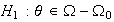 against the alternative
 at level of significance
 .
We want the probability of the incorrect decision when the drift is 20% per
year to be small, so let us choose it to be
.
We want the probability of the incorrect decision when the drift is 20% per
year to be small, so let us choose it to be
 as well, which means that when
 the power of the test should be at least
 How large a sample must be taken in order to insure this?
The test itself is easy to express. We reject the null hypothesis if
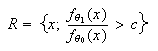 where the value
 has been chosen so that
 when
when
 has a standard normal distribution. The power of the test is the probability
 when the parameter
 and this is
 where
where
 has a standard normal distribution. Since we want the power to be
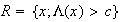 the value
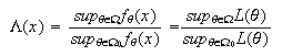 must be chosen to be
 Solving for the value of

 Now if we try some reasonable values for the parameters, for example


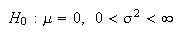 ,
then
,
then
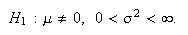 which is about 55 years worth of data, far larger a sample than we could hope
to collect. This example shows that the typical variabilities in the market
are so large, compared with even fairly high rates of return, that it is
almost impossible to distinguish between theoretical rates of return of 0% and
20% per annum using a hypothesis test with daily data.
which is about 55 years worth of data, far larger a sample than we could hope
to collect. This example shows that the typical variabilities in the market
are so large, compared with even fairly high rates of return, that it is
almost impossible to distinguish between theoretical rates of return of 0% and
20% per annum using a hypothesis test with daily data.
Relationship Betweeen Hypothesis Tests and C.I.'s
There is a close relationship between hypothesis tests and confidence
intervals as the following example illustrates. Suppose
 is a random sample from the
N(
is a random sample from the
N( ,1)
distribution and we wish to test the hypothesis
,1)
distribution and we wish to test the hypothesis
 against
 .
The critical region
.
The critical region
 is a size
 critical region which has a corresponding acceptance region
 Note that the hypothesis
 would not be rejected at the
 level if
 or equivalently
 which is a
 C.I. for

Problem
Let
 be a random sample from the
Gamma
be a random sample from the
Gamma distribution. Show that
 is a size
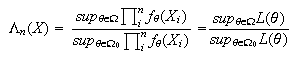 critical region for testing
 .
Show how this critical region may be used to construct a
.
Show how this critical region may be used to construct a
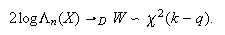 C.I. for

Likelihood Ratio Tests
Consider a test of the hypothesis
 against
 .
We have seen that for prescribed
.
We have seen that for prescribed

 ,
the most powerful test of the simple null hypothesis
,
the most powerful test of the simple null hypothesis
 against a simple alternative
 is based on the likelihood ratio
 .
By the Neyman-Pearson Lemma it has critical region
.
By the Neyman-Pearson Lemma it has critical region
 whre
whre
 is a constant determined by the size of the test. When either the null or the
alternative hypothesis are composite (i.e. contain more than one
point) and there is no uniformly most powerful test, it seems reasonable to
use a test with critical region
is a constant determined by the size of the test. When either the null or the
alternative hypothesis are composite (i.e. contain more than one
point) and there is no uniformly most powerful test, it seems reasonable to
use a test with critical region
 for some choice of
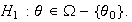 .
The likelihood ratio test does this with
.
The likelihood ratio test does this with
 replaced by
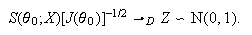 ,
the maximum likelihood estimator over all possible values of the parameter,
and
,
the maximum likelihood estimator over all possible values of the parameter,
and
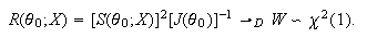 replaced by the maximum likelihood estimator of the parameter when it is
restricted to
replaced by the maximum likelihood estimator of the parameter when it is
restricted to
 .
Thus, the likelihood ratio test has critical region
.
Thus, the likelihood ratio test has critical region
 where
where
 and
and
 is determined by the size of the test. In general, the distribution of the
test statistic
is determined by the size of the test. In general, the distribution of the
test statistic
 may be difficult to find. Fortunately, however, the asymptotic distribution is
known under fairly general conditions. In a few cases, we can show that the
likelihood ratio test is equivalent to the use of a statistic with known
distribution. However, in many cases, we need to rely on the asymptotic
chi-squared distribution of Theorem 4.4.6.
may be difficult to find. Fortunately, however, the asymptotic distribution is
known under fairly general conditions. In a few cases, we can show that the
likelihood ratio test is equivalent to the use of a statistic with known
distribution. However, in many cases, we need to rely on the asymptotic
chi-squared distribution of Theorem 4.4.6.
Example
Let
 be a random sample from the
N
be a random sample from the
N distribution where
 and
and
 are unknown. Consider a test of
 against the alternative
 We can show that the likelihood ratio test of
 against
 has critical region
 .
Under
.
Under
 that the statistic
 has a
F
has a
F distribution and we can thus find a size
 test for
 .
.
Theorem B6
Suppose
 is a random sample from a regular statistical model
 with
with
 an open set in
 dimensional
Euclidean space. Consider a subset of
dimensional
Euclidean space. Consider a subset of
 defined by
 open subset of
 -dimensional
Euclidean space
-dimensional
Euclidean space
 .
Then the likelihood ratio statistic defined by
.
Then the likelihood ratio statistic defined by
 is such that, under the hypothesis
 ,
,
 Note: The number of degrees of freedom is the difference
between the number of parameters that need to be estimated in the general
model, and the number of parameters left to be estimated under the
restrictions imposed by
Note: The number of degrees of freedom is the difference
between the number of parameters that need to be estimated in the general
model, and the number of parameters left to be estimated under the
restrictions imposed by
 .
.
Significance Tests and p-values
We have seen that a test of hypothesis is a rule which allows us to decide
whether to accept the null hypothesis
 or to reject it in favour of the alternative hypothesis
 based
on the observed data. In situations in which
based
on the observed data. In situations in which
 is difficult to specify a test of significance could be used. A (pure) test of
significance is a procedure for measuring the strength of the evidence
provided by the observed data against
is difficult to specify a test of significance could be used. A (pure) test of
significance is a procedure for measuring the strength of the evidence
provided by the observed data against
 .
This method usually involves looking at the distribution of a test statisitic
or discrepancy measure
.
This method usually involves looking at the distribution of a test statisitic
or discrepancy measure
 under
under
 The p-value or significance level for the test is the
probability, computed under
The p-value or significance level for the test is the
probability, computed under
 of observing a
 value at least as extreme as the value observed. The smaller the observed
p-value, the stronger the evidence against
value at least as extreme as the value observed. The smaller the observed
p-value, the stronger the evidence against
 .
The difficulty with this approach is how to find a statistic with `good
properties'. The likelihood ratio statistic provides a general test statistic
which may be used.
.
The difficulty with this approach is how to find a statistic with `good
properties'. The likelihood ratio statistic provides a general test statistic
which may be used.
Score and Wald Tests
Score Test
Score tests can be viewed as a more general class of tests of
 against
 which tend to have considerable power provided that the values of the
parameter under the null and the alternative are close. If the usual
regularity conditions hold then under
which tend to have considerable power provided that the values of the
parameter under the null and the alternative are close. If the usual
regularity conditions hold then under
 we have
 and thus
 For a vector
 we have
 The test based on
 is called a (Rao) score test. It has critical region
 where
where
 is determined by the size of the test, that is,
 satisfies
 where
where
 The test based on
 is asymptotically equivalent to the likelihood ratio test.
Wald Test
Suppose that
 is the maximum likelihood estimator of
 over all
 and we wish to test
 against
 If the usual regularity conditions hold then under

 A
test based on the test statistic
A
test based on the test statistic
 is called a Wald test. It has critical region
 where
where
 is determined by the size of the test. Both the score test and the Wald test
are asymptotically equivalent to the likelihood ratio test and the intuitive
expanation for these equivalences are quite simple. For large values of the
sample size
is determined by the size of the test. Both the score test and the Wald test
are asymptotically equivalent to the likelihood ratio test and the intuitive
expanation for these equivalences are quite simple. For large values of the
sample size
 the maximum likelihood estimator
 is close to the true value of the parameter
 and so the log likelihood can be approximated by the first two terms in the
Taylor series expansion of
and so the log likelihood can be approximated by the first two terms in the
Taylor series expansion of
 about
about
 and so
 since
since
 and
the observed
information
and
the observed
information  is asymptotically equivalent to the Fisher information
 This verifies the equivalence of the likelihood ratio and the Wald test.