 in sample spaces to describe such outcomes. In this chapter we introduce
numerical-valued variables
in sample spaces to describe such outcomes. In this chapter we introduce
numerical-valued variables
 to describe outcomes. This allows probability models to be manipulated easily
using ideas from algebra, calculus, or geometry.
to describe outcomes. This allows probability models to be manipulated easily
using ideas from algebra, calculus, or geometry.
Probability models are used to describe outcomes associated with random
processes. So far we have used sets
in sample spaces to describe such outcomes. In this chapter we introduce
numerical-valued variables
to describe outcomes. This allows probability models to be manipulated easily
using ideas from algebra, calculus, or geometry.
A random variable (r.v.) is a numerical-valued variable that represents
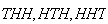
outcomes in an experiment or random process. For example, suppose a coin is
tossed 3 times; then
 would be a random variable. Associated with any random variable is a
range or domain
would be a random variable. Associated with any random variable is a
range or domain
 ,
which is the set of possible values for the variable. For example, the random
variable
,
which is the set of possible values for the variable. For example, the random
variable
 defined above has range
 .
.
Random variables are denoted by capital letters like
 and their possible values are denoted by
 .
This gives a nice short-hand notation for outcomes: for example,
.
This gives a nice short-hand notation for outcomes: for example,
 in the experiment above stands for ``2 heads occurred''.
Random variables are always defined so that if the associated random process
or experiment is carried out, then one and only one of the outcomes
 occurs. In other words, the possible values for
 form a partition of the points in the sample space for the experiment. In more
advanced mathematical treatments of probability, a random variable is defined
as a function on a sample space, as follows:
form a partition of the points in the sample space for the experiment. In more
advanced mathematical treatments of probability, a random variable is defined
as a function on a sample space, as follows:
A random variable is a function that assigns a real number to
each point in a sample space
 .
.
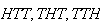
To understand this definition, consider the experiment in which a coin is
tossed 3 times, and suppose that we used the sample space
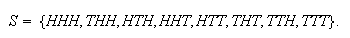 Then each of the outcomes
 (where
 = number of heads) represents an event (either simple or compound) and so a
real number
= number of heads) represents an event (either simple or compound) and so a
real number
 can be associated with each point in
 .
In particular, the point
.
In particular, the point
 corresponds to
 ;
the points
;
the points
 correspond to
 ;
the points
;
the points
 correspond to
 ;
and the point
;
and the point
 corresponds to
 .
.
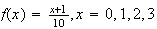
As you may recall, a function is a mapping of each point in a domain into a
unique point. e.g. The function
 maps the point
 in the domain into the point
 in the range. We are familiar with this rule for mapping being defined by a
mathematical formula. However, the rule for mapping a point in the sample
space (domain) into the real number in the range of a random variable is most
often given in words rather than by a formula. As mentioned above, we
generally denote random variables, in the abstract, by capital letters
in the range. We are familiar with this rule for mapping being defined by a
mathematical formula. However, the rule for mapping a point in the sample
space (domain) into the real number in the range of a random variable is most
often given in words rather than by a formula. As mentioned above, we
generally denote random variables, in the abstract, by capital letters
 ,
etc.) and denote the actual numbers taken by random variables by small letters
,
etc.) and denote the actual numbers taken by random variables by small letters
 ,
etc.). You may, in your earlier studies, have had this distinction made
between a function
,
etc.). You may, in your earlier studies, have had this distinction made
between a function
 and the value of a function
 .
.
Since
 represents an outcome of some kind, we will be interested in its probability,
which we write as
represents an outcome of some kind, we will be interested in its probability,
which we write as
 .
To discuss probabilities for random variables, it is easiest if they are
classified into two types, according to their ranges:
.
To discuss probabilities for random variables, it is easiest if they are
classified into two types, according to their ranges:
Discrete r.v.'s take integer values or, more generally, values in a countable set (recall that a set is countable if its elements can be placed in a one-one correspondence with a subset of the positive integers).
Continuous r.v.'s take values in some interval of real
numbers.
Examples might be:
| Discrete | Continuous |
| number of people in a car | total weight of people in a car |
| number of cars in a parking lot | distance between cars in a parking lot |
| number of phone calls to 911 | time between calls to 911. |
In theory there could also be mixed r.v.'s which are discrete-valued over part of their range and continuous-valued over some other portion of their range. We will ignore this possibility here and concentrate first on discrete r.v.'s. Continuous r.v.'s are considered in Chapter 9.
Our aim is to set up general models which describe how the probability is
distributed among the possible values a random variable can take. To do this
we define for any discrete random variable
 the probability function.
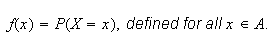
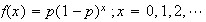
The probability function (p.f.) of a random variable
 is the function
The set of pairs
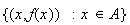 is called the probability distribution of
 .
All probability functions must have two properties:
.
All probability functions must have two properties:
 for all values of
 (i.e. for
 )
)

By implication, these properties ensure that
 for all
 .
We consider a few ``toy'' examples before dealing with more complicated
problems.
.
We consider a few ``toy'' examples before dealing with more complicated
problems.
Example 1: Let
 be the number obtained when a die is thrown. We would normally use the
probability function
be the number obtained when a die is thrown. We would normally use the
probability function
 for
for
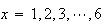 .
In fact there probably is no absolutely perfect die in existence. For most
dice, however, the 6 sides will be close enough to being equally likely that
.
In fact there probably is no absolutely perfect die in existence. For most
dice, however, the 6 sides will be close enough to being equally likely that
 is a satisfactory model for the distribution of probability among the possible
outcomes.
is a satisfactory model for the distribution of probability among the possible
outcomes.
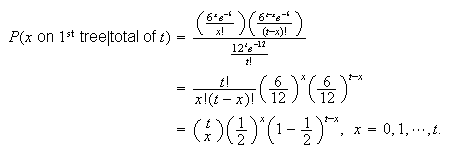
Example 2: Suppose a "fair" coin is tossed 3 times, and let
 be the number of heads occurring. Then a simple calculation using the ideas
from earlier chapters gives
be the number of heads occurring. Then a simple calculation using the ideas
from earlier chapters gives
 Note that instead of writing
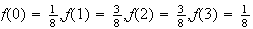 ,
we have given a simple algebraic
expression.
,
we have given a simple algebraic
expression.
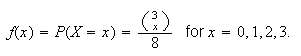
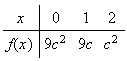
Example 3: Find the value of
 which makes
 below a probability function.
 |
0 | 1 | 2 | 3 |
 |
 |
 |
 |
 |
Using
 gives
gives
 .
Hence
.
Hence
 .
.
While the probability function is the most common way of describing a probability model, there are other possibilities. One of them is by using the cumulative distribution function (c.d.f.).
The cumulative distribution function of
 is the function usually denoted by

 defined for all real numbers
 .
.
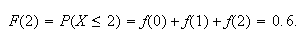
In the last example, with
 ,
we have for
,
we have for

 |
0 | 1 | 2 | 3 |
 |
0.1 | 0.3 | 0.6 | 1 |
since, for instance,
 Similarly,
 can be defined for real numbers
 not in the range of the random variable, for example
 The c.d.f. for this example is plotted in Figure
cdf.
The c.d.f. for this example is plotted in Figure
cdf.
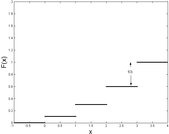
A simple cumulative
distribution function
In general,
 can be obtained from
 by the fact that
A c.d.f.
 has certain properties, just as a probability function
 does. Obviously, since it represents a probability,
 must be between 0 and 1. In addition it must be a non-decreasing function
(e.g.
must be between 0 and 1. In addition it must be a non-decreasing function
(e.g.
 cannot be less than
 ).
Thus we note the following properties of a c.d.f.
).
Thus we note the following properties of a c.d.f.
 :
:
 is a non-decreasing function of

 for all

 and
and
We have noted above that
 can be obtained from
 .
The opposite is also true; for example the following result holds:
.
The opposite is also true; for example the following result holds:
If
 takes
on integer values then for values
takes
on integer values then for values
 such
that
such
that
 and
and
 ,
,
 This says that
 is the size of the jump in
 at the point

To prove this, just note that

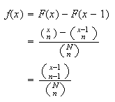
When a random variable has been defined it is sometimes simpler to find its
probability function (p.f.)
 first, and sometimes it is simpler to find
 first. The following example gives two approaches for the same
problem.
first. The following example gives two approaches for the same
problem.
Example: Suppose that
 balls labelled
 are placed in a box, and
 balls
balls
 are randomly selected without replacement. Define the r.v.
 Find the probability function for
 .
.
Solution 1: If
 then we must select the number
 plus
plus
 numbers from the set
 .
(Note that this means we need
.
(Note that this means we need
 .)
This gives
.)
This gives
Solution 2: First find
 .
Noting that
.
Noting that
 if and only if all
 balls selected are from the set
 ,
we get
,
we get
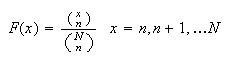 We can now find
 as before.
Remark: When you write down a probability function or a cumulative distribution function, don't forget to give the range of the function (i.e. the possible values of the random variable). This is part of the function's definition.
Sometimes we want to graph a probability function
 .
The type of graph we will use most is called a (probability)
histogram. For now, we'll define this only for r.v.'s whose
range is some set of consecutive integers
.
The type of graph we will use most is called a (probability)
histogram. For now, we'll define this only for r.v.'s whose
range is some set of consecutive integers
 .
A histogram of
.
A histogram of
 is then a graph consisting of adjacent bars or rectangles. At each
 we place a rectangle with base on
 and with height
 .
In the above Example 3, a histogram of
.
In the above Example 3, a histogram of
 looks like that in Figure
probhist.
looks like that in Figure
probhist.
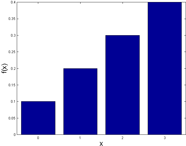
Probability histogram for
Notice that the areas of these rectangles correspond to the probabilities, so
for example
 is the sum of the area of the three rectangles above the points
 and
and
 In general, probabilities are depicted by areas.
Model Distributions:
Many processes or problems have the same structure. In the remainder of this course we will identify common types of problems and develop probability distributions that represent them. In doing this it is important to be able to strip away the particular wording of a problem and look for its essential features. For example, the following three problems are all essentially the same.
A fair coin is tossed 10 times and the ``number of heads obtained''
 is recorded.
Twenty seeds are planted in separate pots and the ``number of seeds
germinating''
 is recorded.
Twelve items are picked at random from a factory's production line and
examined for defects. The number of items having no defects
 is recorded.
What are the common features? In each case the process consists of ``trials" which are repeated a stated number of times - 10, 20, and 12. In each repetition there are two types of outcomes - heads/tails, germinate/don't germinate, and no defects/defects. These repetitions are independent (as far as we can determine), with the probability of each type of outcome remaining constant for each repetition. The random variable we record is the number of times one of these two types of outcome occurred.
Six model distributions for discrete r.v.'s will be developed in the rest of
this chapter. Students often have trouble deciding which one (if any) to use
in a given setting, so be sure you understand the physical setup which leads
to each one. Also, as illustrated above you will need to learn to focus on the
essential features of the situation as well as the particular content of the
problem.
Statistical Computing
A number of major software systems have been developed for probability and
statistics. We will use a system called
 ,
which has a wide variety of features and which has Unix and Windows versions.
Appendix 6.1 at the end of this chapter gives a brief introduction to
,
which has a wide variety of features and which has Unix and Windows versions.
Appendix 6.1 at the end of this chapter gives a brief introduction to
 ,
and how to access it. For this course,
,
and how to access it. For this course,
 can compute probabilities for all the distributions we consider, can graph
functions or data, and can simulate random processes. In the sections below we
will indicate how
can compute probabilities for all the distributions we consider, can graph
functions or data, and can simulate random processes. In the sections below we
will indicate how
 can be used for some of these tasks.
Problems:
Let
 have probability function
 .
Find
.
Find
 .
.
Suppose that 5 people, including you and a friend, line up at random. Let
 be the number of people standing between you and your friend. Tabulate the
probability function and the cumulative distribution function for
be the number of people standing between you and your friend. Tabulate the
probability function and the cumulative distribution function for
 .
.
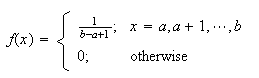
We define each model in terms of an abstract ``physical setup", or setting, and then consider specific examples of the setup.
Physical Setup: Suppose
 takes values
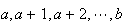 with all values being equally likely. Then
 has a discrete uniform distribution, on
![$[a,b]$](graphics/noteschap6__150.png) .
.
Illustrations:
If
 is the number obtained when a die is rolled, then
 has a discrete uniform distribution with
 and
and
 .
.
Computer random number generators give uniform
![$[1,N]$](graphics/noteschap6__155.png) variables, for a specified positive integer
variables, for a specified positive integer
 .
These are used for many purposes, e.g. generating lottery numbers or providing
automated random sampling from a set of
.
These are used for many purposes, e.g. generating lottery numbers or providing
automated random sampling from a set of
 items.
Probability Function: There are
 values
 can take so the probability at each of these values must be
 in order that
 .
Therefore
.
Therefore
Problem 6.2.1
Let
 be the largest number when a die is rolled 3 times. First find the c.d.f.,
 ,
and then find the probability function,
,
and then find the probability function,
 .
.
Physical Setup: We have a collection of
 objects which can be classified into two distinct types. Call one type
"success" Note_1
objects which can be classified into two distinct types. Call one type
"success" Note_1  and the other type
"failure"
and the other type
"failure"  .
There are
.
There are
 successes and
 failures. Pick
 objects at random without replacement. Let
 be the number of successes obtained. Then
 has a hypergeometric distribution.
Illustrations:
The number of aces
 in a bridge hand has a hypergeometric distribution with
 ,
and
,
and
 .
.
In a fleet of 200 trucks there are 12 which have defective brakes. In a safety
check 10 trucks are picked at random for inspection. The number of trucks
 with defective brakes chosen for inspection has a hypergeometric distribution
with
with defective brakes chosen for inspection has a hypergeometric distribution
with
 .
.
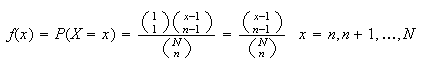
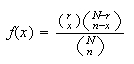
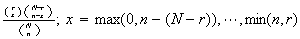
Probability Function: Using counting techniques we note
there are
 points in the sample space
 if we don't consider order of selection. There are
 ways to choose the
 success objects from the
 available and
 ways to choose the remaining
 objects from the
 failures. Hence
 The range of values for
 is somewhat complicated. Of course,
 .
However if the number,
.
However if the number,
 ,
picked exceeds the number,
,
picked exceeds the number,
 ,
of failures, the difference,
,
of failures, the difference,
 must be successes. So
 .
Also,
.
Also,
 since we can't get more successes than the number available. But
 ,
since we can't get more successes than the number of objects chosen.
,
since we can't get more successes than the number of objects chosen.
 .
.
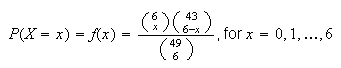
Example: In Lotto 6/49 a player selects a set of six
numbers (with no repeats) from the set
 .
In the lottery draw six numbers are selected at random. Find the probability
function for
.
In the lottery draw six numbers are selected at random. Find the probability
function for
 ,
the number from your set which are drawn.
,
the number from your set which are drawn.
Solution: Think of your numbers as the
 objects and the remainder as the
 objects. Then
 has a hypergeometric distribution with
 and
and
 ,
so
,
so
 For example, you win the jackpot prize if
 ;
the probability of this is
;
the probability of this is
 ,
or about 1 in 13.9 million.
,
or about 1 in 13.9 million.
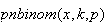
Remark: Hypergeometric probabilities are tedious to compute
using a calculator. The
 functions
 and
and
 can be used to evaluate
 and the c.d.f
 .
In particular,
.
In particular,
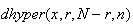 gives
gives
 and
and
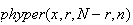 gives
gives
 .
Using this we find for the Lotto 6/49 problem here, for example, that
.
Using this we find for the Lotto 6/49 problem here, for example, that
 is calculated by typing
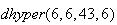 in
in
 ,
which returns the answer
,
which returns the answer
 or
or
 .
.
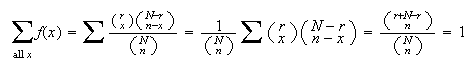
For all of our model distributions we can also confirm that
 .
To do this here we use a summation result from Chapter 5 called the
hypergeometric identity. Letting
.
To do this here we use a summation result from Chapter 5 called the
hypergeometric identity. Letting
 in that identity we get
Problems:
A box of 12 tins of tuna contains
 which are tainted. Suppose 7 tins are opened for inspection and none of these
7 is tainted.
which are tainted. Suppose 7 tins are opened for inspection and none of these
7 is tainted.
Calculate the probability that none of the 7 is tainted for
 .
.
Do you think it is likely that the box contains as many as 3 tainted tins?
Derive a formula for the hypergeometric probability function using a sample space in which order of selection is considered.
Physical Setup:
Suppose an "experiment" has two types of distinct outcomes. Call these types
"success"  and
"failure"
and
"failure"  ,
and let their probabilities be
,
and let their probabilities be
 (for
(for
 )
and
)
and
 (for
(for
 ).
Repeat the experiment
).
Repeat the experiment
 independent times. Let
 be the number of successes obtained. Then
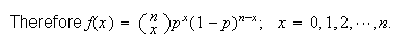
 has what is called a binomial distribution. (We write
 as a shorthand for
"
as a shorthand for
" is distributed according to a binomial distribution with
 repetitions and probability
 of success".) The individual experiments in the process just described are
often called "trials", and the process is called a
Bernoulli Note_2 process or a
binomial process.
of success".) The individual experiments in the process just described are
often called "trials", and the process is called a
Bernoulli Note_2 process or a
binomial process.
Illustrations:
Toss a fair die 10 times and let
 be the number of sixes that occur. Then
 .
.
In a microcircuit manufacturing process, 60% of the chips produced work (40%
are defective). Suppose we select 25 independent chips and let
 be the number that work. Then
 .
.
Comment: We must think carefully whether the physical
process we are considering is closely approximated by a binomial process, for
which the key assumptions are that (i) the probability
 of success is constant over the
 trials, and (ii) the outcome
(
trials, and (ii) the outcome
( or
or
 )
on any trial is independent of the outcome on the other trials. For
Illustration 1 these assumptions seem appropriate. For Illustration 2 we would
need to think about the manufacturing process. Microcircuit chips are produced
on "wafers" containing a large number of chips and it is common for defective
chips to cluster on wafers. This could mean that if we selected 25 chips from
the same wafer, or from only 2 or 3 wafers, that the "trials" (chips) might
not be independent.
)
on any trial is independent of the outcome on the other trials. For
Illustration 1 these assumptions seem appropriate. For Illustration 2 we would
need to think about the manufacturing process. Microcircuit chips are produced
on "wafers" containing a large number of chips and it is common for defective
chips to cluster on wafers. This could mean that if we selected 25 chips from
the same wafer, or from only 2 or 3 wafers, that the "trials" (chips) might
not be independent.
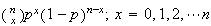
Probability Function: There are
 different arrangements of

 's
and
's
and
 's
over the
's
over the
 trials. The probability for each of these arrangements has
 multiplied together
 times and
 multiplied
 times, in some order, since the trials are independent. So each arrangement
has probability
times, in some order, since the trials are independent. So each arrangement
has probability
 .
.
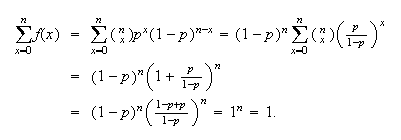
 Checking that
 :
:
 We graph in Figure binomhist the probability function
for the Binomial distribution with parameters
We graph in Figure binomhist the probability function
for the Binomial distribution with parameters
 and
and
 Although the formula for
 may seem complicated this shape is typically, increasing to a maximum value
near
may seem complicated this shape is typically, increasing to a maximum value
near
 and then decreasing thereafter.
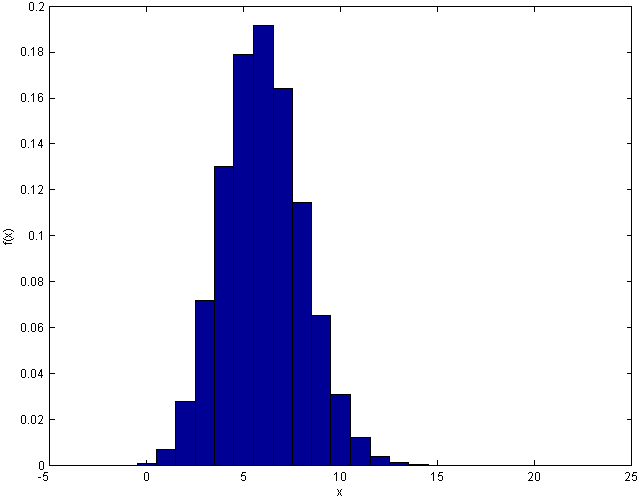
The
Binomial
 probability histogram.
Computation: Many software packages and some calculators
give binomial probabilities. In
 we use the function
 to compute
 and
and
 to compute the corresponding c.d.f.
 .
.
Example Suppose that in a weekly lottery you have
probability .02 of winning a prize with a single ticket. If you buy 1 ticket
per week for 52 weeks, what is the probability that (a) you win no prizes, and
(b) that you win 3 or more prizes?
Solution: Let
 be the number of weeks that you win; then
 .
We find
.
We find

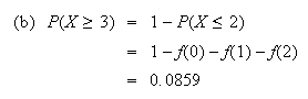
(Note
that
 is given by the
 command
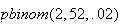 .)
.)
Comparison
of Binomial and Hypergeometric Distributions:
These distributions are similar in that an experiment with 2 types of outcome
( and
and
 )
is repeated
)
is repeated
 times and
 is the number of successes. The key difference is that the binomial requires
independent repetitions with the same probability of
is the number of successes. The key difference is that the binomial requires
independent repetitions with the same probability of
 ,
whereas the draws in the hypergeometric are made from a fixed collection of
objects without replacement. The trials (draws) are therefore
not independent. For example, if there are
,
whereas the draws in the hypergeometric are made from a fixed collection of
objects without replacement. The trials (draws) are therefore
not independent. For example, if there are

 objects and

 objects, then the probability of getting an
 on draw 2 depends on what was obtained in draw 1. If these draws had been made
with replacement, however, they would be independent and we'd
use the binomial rather than the hypergeometric model.
on draw 2 depends on what was obtained in draw 1. If these draws had been made
with replacement, however, they would be independent and we'd
use the binomial rather than the hypergeometric model.
If
 is large and the number,
 ,
being drawn is relatively small in the hypergeometric setup then we are
unlikely to get the same object more than once even if we do replace it. So it
makes little practical difference whether we draw with or without replacement.
This suggests that when we are drawing a fairly small proportion of a large
collection of objects the binomial and the hypergeometric models should
produce similar probabilities. As the binomial is easier to calculate, it is
often used as an approximation to the hypergeometric in such
cases.
,
being drawn is relatively small in the hypergeometric setup then we are
unlikely to get the same object more than once even if we do replace it. So it
makes little practical difference whether we draw with or without replacement.
This suggests that when we are drawing a fairly small proportion of a large
collection of objects the binomial and the hypergeometric models should
produce similar probabilities. As the binomial is easier to calculate, it is
often used as an approximation to the hypergeometric in such
cases.
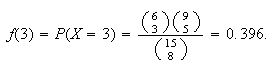
Example: Suppose we have 15 cans of soup with no labels,
but 6 are tomato and 9 are pea soup. We randomly pick 8 cans and open them.
Find the probability 3 are tomato.
Solution: The correct solution uses hypergeometric, and is
(with
 = number of tomato soups picked)
 If we incorrectly used binomial, we'd get
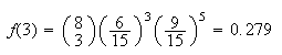 As expected, this is a poor approximation since we're picking over half of a
fairly small collection of cans.
As expected, this is a poor approximation since we're picking over half of a
fairly small collection of cans.
However, if we had 1500 cans - 600 tomato and 900 pea, we're not likely to get
the same can again even if we did replace each of the 8 cans after opening it.
(Put another way, the probability we get a tomato soup on each pick is very
close to .4, regardless of what the other picks give.) The exact,
hypergeometric, probability is now
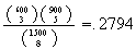 .
Here the binomial probability,
.
Here the binomial probability,
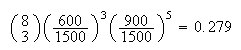 is a very good approximation.
Problems:
Megan audits 130 clients during a year and finds irregularities for 26 of them.
Give an expression for the probability that 2 clients will have irregularities when 6 of her clients are picked at random,
Evaluate your answer to (a) using a suitable approximation.
The flash mechanism on camera
 fails on 10% of shots, while that of camera
 fails on 5% of shots. The two cameras being identical in appearance, a
photographer selects one at random and takes 10 indoor shots using the flash.
fails on 5% of shots. The two cameras being identical in appearance, a
photographer selects one at random and takes 10 indoor shots using the flash.
Give the probability that the flash mechanism fails exactly twice. What assumption(s) are you making?
Given that the flash mechanism failed exactly twice, what is the probability
camera
 was selected?
Physical Setup:
The setup for this distribution is almost the same as for binomial; i.e. an
experiment (trial) has two distinct types of outcome
( and
and
 )
and is repeated independently with the same probability,
)
and is repeated independently with the same probability,
 ,
of success each time. Continue doing the experiment until a specified number,
,
of success each time. Continue doing the experiment until a specified number,
 ,
of success have been obtained. Let
,
of success have been obtained. Let
 be the number of failures obtained before the
 success. Then
 has a negative binomial distribution. We often write
 to denote this.
Illustrations:
If a fair coin is tossed until we get our
 head, the number of tails we obtain has a negative binomial distribution with
 and
and
 .
.
As a rough approximation, the number of half credit failures a student
collects before successfully completing 40 half credits for an honours degree
has a negative binomial distribution. (Assume all course attempts are
independent, with the same probability of being successful, and ignore the
fact that getting more than 6 half credit failures prevents a student from
continuing toward an honours degree.)
Probability Function: In all there will be
 trials
(
trials
(
 's
and
's
and

 's)
and the last trial must be a success. In the first
's)
and the last trial must be a success. In the first
 trials we therefore need
 failures and
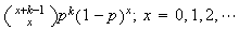
 successes, in any order. There are
 different orders. Each order will have probability
 since there must be
 trials which are failures and
 which are success. Hence
Note: An alternate version of the negative binomial
distribution defines
 to be the total number of trials needed to get the
 success. This is equivalent to our version. For example, asking for the
probability of getting 3 tails before the
success. This is equivalent to our version. For example, asking for the
probability of getting 3 tails before the
 head is exactly the same as asking for a total of 8 tosses in order to get the
 head. You need to be careful to read how
 is defined in a problem rather than mechanically "plugging in" numbers in the
above formula for
is defined in a problem rather than mechanically "plugging in" numbers in the
above formula for
 .
.
Checking that
 requires somewhat more work for the negative binomial distribution. We first
re-arrange the
requires somewhat more work for the negative binomial distribution. We first
re-arrange the
 term,
term,
 Factor a (-1) out of each of the
 terms in the numerator, and re-write these terms in reverse
order,
terms in the numerator, and re-write these terms in reverse
order, Then (using the binomial
theorem)
Then (using the binomial
theorem)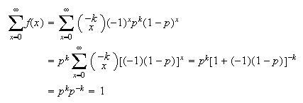
Comparison of Binomial and Negative Binomial
Distributions
These should be easily distinguished because they reverse what is specified or known in advance and what is variable.
| Binomial: | Know the number,
 ,
of repetitions in advance. Don't know the number of successes we'll obtain
until after the experiment. ,
of repetitions in advance. Don't know the number of successes we'll obtain
until after the experiment. |
| Negative Binomial: | Know the number,
 ,
of successes in advance. Don't know the number of repetitions needed until
after the experiment. ,
of successes in advance. Don't know the number of repetitions needed until
after the experiment. |
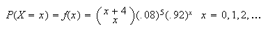
Example:
The fraction of a large population that has a specific blood type
 is .08 (8%). For blood donation purposes it is necessary to find 4 people with
type
is .08 (8%). For blood donation purposes it is necessary to find 4 people with
type
 blood. If randomly selected individuals from the population are tested one
after another, then (a) What is the probability
blood. If randomly selected individuals from the population are tested one
after another, then (a) What is the probability
 persons have to be tested to get 5 type
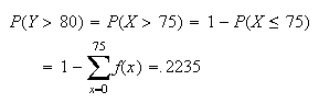
 persons, and (b) What is the probability that over 80 people have to be
tested?
persons, and (b) What is the probability that over 80 people have to be
tested?
Solution:
Think of a type
 person as a success
 and a non-type
 as an
as an
 .
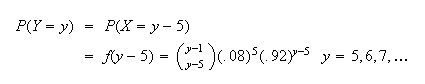
Let
.
Let
 = number of persons who have to be tested and let
 = number of non-type
 persons in order to get 5
 's.
Then
's.
Then
 and
and
 We are actually asked here about
 .
Thus
.
Thus
 Thus we have the answer to (a) as given above, and
(b)
Note: Calculating such probabilities is easy with
 .
To get
.
To get
 we use
 and to get
 we use
 .
.
Problems:
You can get a group rate on tickets to a play if you can find 25 people to go.
Assume each person you ask responds independently and has a 20% chance of
agreeing to buy a ticket. Let
 be the total number of people you have to ask in order to find 25 who agree to
buy a ticket. Find the probability function of
be the total number of people you have to ask in order to find 25 who agree to
buy a ticket. Find the probability function of
 .
.
A shipment of 2500 car headlights contains 200 which are defective. You choose
from this shipment without replacement until you have 18 which are not
defective. Let
 be the number of defective headlights you obtain.
Give the probability function,
 .
.
Using a suitable approximation, find
 .
.
Physical Setup:
This is a special case of the negative binomial distribution with
 ,
i.e., an experiment is repeated independently with two types of outcome
(
,
i.e., an experiment is repeated independently with two types of outcome
( and
and
 )
each time, and the same probability,
)
each time, and the same probability,
 ,
of success each time. Let
,
of success each time. Let
 be the number of failures obtained before the first success.
Illustrations:
The probability you win a lottery prize in any given week is a constant
 .
The number of weeks before you win a prize for the first time
has a geometric distribution.
.
The number of weeks before you win a prize for the first time
has a geometric distribution.
If you take STAT 230 until you pass it and attempts are independent with the
same probability of a pass each time, then the number of failures would have a
geometric distribution. (These assumptions are unlikely to be true for most
persons! Why is this?)
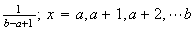
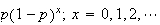
Probability Function:
There is only the one arrangement with
 failures followed by 1 success. This arrangement has probability
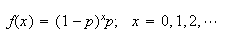 which is the same as
 for
for
 .
.
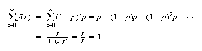
Checking that
 ,
we will be evaluating a geometric series,
,
we will be evaluating a geometric series,
Note: The names of the models so far derive from the
summation results which show
 sums to 1. The geometric distribution involved a geometric series; the
hypergeometric distribution used the hypergeometric identity; both the
binomial and negative binomial distributions used the binomial
theorem.
sums to 1. The geometric distribution involved a geometric series; the
hypergeometric distribution used the hypergeometric identity; both the
binomial and negative binomial distributions used the binomial
theorem.
Bernoulli Trials
The binomial, negative binomial and
geometric models involve trials (experiments) which:
| (1) | are independent |
| (2) | have 2 distinct types of outcome
( and
and
 ) ) |
| (3) | have the same probability of ``success''
 each time.
 |
Such trials are known as Bernoulli trials; they are named after an 18th
century mathematician.
Problem 6.6.1
Suppose there is a 30% chance of a car from a certain production line having a
leaky windshield. The probability an inspector will have to check at least
 cars to find the first one with a leaky windshield is .05. Find
 .
.
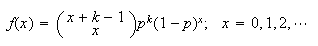
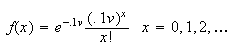
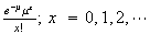
The Poisson Note_3
distribution has probability function (p.f.) of the form
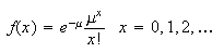 where
where
 is a parameter whose value depends on the setting for the model.
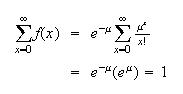
Mathematically, we can see that
is a parameter whose value depends on the setting for the model.
Mathematically, we can see that
 has the properties of a p.f., since
 for
for
 and since
 The Poisson distribution arises in physical settings where the random variable
 represents the number of events of some type. In this section we show how it
arises from a binomial process, and in the following section we consider
another derivation of the model.
represents the number of events of some type. In this section we show how it
arises from a binomial process, and in the following section we consider
another derivation of the model.
We will sometimes write
 to denote that
 has the p.f. above.
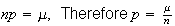
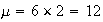
Physical Setup: One way the Poisson distribution arises is
as a limiting case of the binomial distribution as
 and
and
 .
In particular, we keep the product
.
In particular, we keep the product
 fixed at some constant value,
 ,
while letting
,
while letting
 .
This automatically makes
.
This automatically makes
 .
Let us see what the limit of the binomial p.f.
.
Let us see what the limit of the binomial p.f.
 is in this case.
Probability Function: Since
 and
and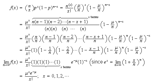 (For the binomial the upper limit on
 is
is
 ,
but we are letting
,
but we are letting
 .)
This result allows us to use the Poisson distribution with
.)
This result allows us to use the Poisson distribution with
 as a close approximation to the binomial distribution
 in processes for which
 is large and
 is small.
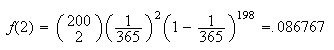
Example: 200 people are at a party. What is the probability
that 2 of them were born on Jan. 1?
Solution: Assuming all days of the year are equally likely
for a birthday (and ignoring February 29) and that the birthdays are
independent (e.g. no twins!) we can use the binomial distribution with
 and
and
 for
for
 = number born on January 1, giving
 Since
Since
 is large and
 is close to 0, we can use the Poisson distribution to approximate this
binomial probability, with
is close to 0, we can use the Poisson distribution to approximate this
binomial probability, with
 ,
giving
,
giving
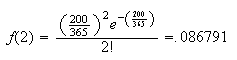 As might be expected, this is a very good approximation.
Notes:
If
 is close to 1 we can also use the Poisson distribution to approximate the
binomial. By interchanging the labels ``success'' and ``failure'', we can get
the probability of ``success'' (formerly labelled ``failure'') close to 0.
is close to 1 we can also use the Poisson distribution to approximate the
binomial. By interchanging the labels ``success'' and ``failure'', we can get
the probability of ``success'' (formerly labelled ``failure'') close to 0.
The Poisson distribution used to be very useful for approximating binomial
probabilities with
 large and
 near 0 since the calculations are easier. (This assumes values of
 to be available.) With the advent of computers, it is just as easy to
calculate the exact binomial probabilities as the Poisson probabilities.
However, the Poisson approximation is useful when employing a calculator
without a built in binomial function.
to be available.) With the advent of computers, it is just as easy to
calculate the exact binomial probabilities as the Poisson probabilities.
However, the Poisson approximation is useful when employing a calculator
without a built in binomial function.
The
 functions
 and
and
 give
give
 and
and
 .
.
Problem 6.7.1
An airline knows that 97% of the passengers who buy tickets for a certain flight will show up on time. The plane has 120 seats.
They sell 122 tickets. Find the probability that more people will show up than can be carried on the flight. Compare this answer with the answer given by the Poisson approximation.
What assumptions does your answer depend on? How well would you expect these assumptions to be met?
We now derive the Poisson distribution as a model for the number of events of
some type (e.g. births, insurance claims, web site hits) that occur in time or
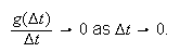
in space. To this end, we use the ``order'' notation
 as
as
 to mean that the function
 approaches
 faster than
 as
as
 approaches zero, or that
 For example
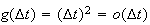 but
but
 is not

Physical Setup:
Consider a situation in which events are occurring randomly over time (or space) according to the following conditions:
Independence: the number of occurrences in non-overlapping intervals are independent.
Individuality: for sufficiently short time periods of length
 the probability of 2 or more events occurring in the interval is close to zero
i.e. events occur singly not in clusters. More precisely, as
the probability of 2 or more events occurring in the interval is close to zero
i.e. events occur singly not in clusters. More precisely, as
 the probability of two or more events in the interval of length
 must go to zero faster than
 or that

Homogeneity or Uniformity: events occur at a uniform or homogeneous rate
 over time so that the probability of one occurrence in an interval
 is approximately
 for small
 for any value of
 More precisely,
These three conditions together define a Poisson Process.
Let
 be the number of event occurrences in a time period of length
 .
Then it can be shown (see below) that
.
Then it can be shown (see below) that
 has a Poisson distribution with
 .
.
Illustrations:
The emission of radioactive particles from a substance follows a Poisson process. (This is used in medical imaging and other areas.)
Hits on a web site during a given time period often follow a Poisson process.
Occurrences of certain non-communicable diseases sometimes follow a Poisson
process.
Probability Function: We can derive the probability
function
 from the conditions above. We are interested in time intervals of arbitrary
length
from the conditions above. We are interested in time intervals of arbitrary
length
 ,
so as a temporary notation, let
,
so as a temporary notation, let
 be the probability of
 occurrences in a time interval of length
 .
We now relate
.
We now relate
 and
and
 .
From that we can determine what
.
From that we can determine what
 is.
is.
To find
 we note that for
 small there are only 2 ways to get
 event occurrences by time
 .
Either there are
.
Either there are
 events by time
 and no more from
 to
to
 or there are
 by time
 and 1 more from
 to
to
 .
(
.
( ,
other possibilities are negligible if
,
other possibilities are negligible if
 is small). This and condition 1 above (independence) imply that
 Re-arranging gives
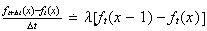 .
.
Taking the limit as
 we get
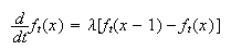 This ``differential-difference" equation can be ``solved" by using the
``boundary" conditions
This ``differential-difference" equation can be ``solved" by using the
``boundary" conditions
 and
and
 for
for
 .
You can confirm that
.
You can confirm that
 satisfies these conditions and the equation above, even though you don't know
how to solve the equations. If we let
satisfies these conditions and the equation above, even though you don't know
how to solve the equations. If we let
 ,
we can re-write
,
we can re-write
 as
as
 ,
which is the Poisson distribution from Section 6.7. That is:
,
which is the Poisson distribution from Section 6.7. That is:
In a Poisson process with rate of occurrence
 ,
the number of event occurrences ,
the number of event occurrences
 |
in a time interval of length
 has a Poisson distribution with
 . . |
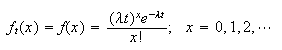
Interpretation of
 and
and
 :
:
 is referred to as the intensity or rate of occurrence
parameter for the events. It represents the average rate of occurrence of
events per unit of time (or area or volume, as discussed below). Then
is referred to as the intensity or rate of occurrence
parameter for the events. It represents the average rate of occurrence of
events per unit of time (or area or volume, as discussed below). Then
 represents the average number of occurrences in
 units of time. It is important to note that the value of
 depends on the units used to measure time. For example, if phone calls arrive
at a store at an average rate of 20 per hour, then
depends on the units used to measure time. For example, if phone calls arrive
at a store at an average rate of 20 per hour, then
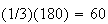
 when time is in hours and the average in 3 hours will be
 or 60. However, if time is measured in minutes then
 ;
the average in 180 minutes (3 hours) is still
;
the average in 180 minutes (3 hours) is still
 .
.
Examples:
Suppose earthquakes recorded in Ontario each year follow a Poisson process
with an average of 6 per year. The probability that 7 earthquakes will be
recorded in a 2 year period is
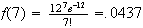 .
We have used
.
We have used
 and
and
 to get
 .
.
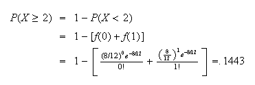
At a nuclear power station an average of 8 leaks of heavy water are reported per year. Find the probability of 2 or more leaks in 1 month, if leaks follow a Poisson process.
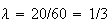
Solution: Assuming leaks satisfy the conditions for a
Poisson process and that a month is
 of a year, we'll use the Poisson distribution with
 and
and
 ,
so
,
so
 .
Thus
.
Thus
Random Occurrence of Events in Space
The Poisson process also applies when ``events'' occur randomly in space
(either 2 or 3 dimensions). For example, the ``events'' might be bacteria in a
volume of water or blemishes in the finish of a paint job on a metal surface.
If
 is the number of events in a volume or area in space of size
 and if
 is the average number of events per unit volume (or area), then
 has a Poisson distribution with
 .
.
For this model to be valid, it
is assumed that the Poisson process conditions given previously apply here,
with ``time'' replaced by ``volume'' or ``area''. Once again, note that the
value of
 depends on the units used to measure volume or area.
Example: Coliform bacteria occur in river water with an
average intensity of 1 bacteria per 10 cubic centimeters (cc) of water. Find
(a) the probability there are no bacteria in a 20cc sample of water which is
tested, and (b) the probability there are 5 or more bacteria in a 50cc sample.
(To do this assume that a Poisson process describes the location of bacteria
in the water at any given time.)
Solution: Let
 = number of bacteria in a sample of volume
 cc. Since
 = 0.1 bacteria per cc (1 per 10cc) the p.f. of
 is Poisson with
 ,
,
 Thus we find
With

With
 and
and

(Note: we can use the
 command
 to get
 .)
.)
Exercise: In each of the above examples, how well are each of the conditions for a Poisson process likely to be satisfied?
Distinguishing Poisson from Binomial and Other Distributions
Students often have trouble knowing when to use the Poisson distribution and when not to use it. To be certain, the 3 conditions for a Poisson process need to be checked. However, a quick decision can often be made by asking yourself the following questions:
Can we specify in advance the maximum value which
 can take?
If we can, then the distribution is not Poisson. If
there is no fixed upper limit, the distribution might be Poisson, but is
certainly not binomial or hypergeometric, e.g. the number of seeds which
germinate out of a package of 25 does not have a Poisson distribution since we
know in advance that
 .
The number of cardinals sighted at a bird feeding station in a week might be
Poisson since we can't specify a fixed upper limit on
.
The number of cardinals sighted at a bird feeding station in a week might be
Poisson since we can't specify a fixed upper limit on
 .
At any rate, this number would not have a binomial or hypergeometric
distribution.
.
At any rate, this number would not have a binomial or hypergeometric
distribution.
Does it make sense to ask how often the event did not occur?
If it
does make sense, the distribution is not Poisson. If it does not make sense,
the distribution might be Poisson. For example, it does not make sense to ask
how often a person did not hiccup during an hour. So the number of hiccups in
an hour might have a Poisson distribution. It would certainly not be binomial,
negative Binomial, or hypergeometric. If a coin were tossed until the
 head occurs it does make sense to ask how often heads did not come up. So the
distribution would not be Poisson. (In fact, we'd use negative binomial for
the number of non-heads; i.e. tails.)
head occurs it does make sense to ask how often heads did not come up. So the
distribution would not be Poisson. (In fact, we'd use negative binomial for
the number of non-heads; i.e. tails.)
Problems:
Suppose that emergency calls to 911 follow a Poisson process with an average of 3 calls per minute. Find the probability there will be
6 calls in a period of
2 minutes.
2 calls in the first minute of a
2 minute period, given that 6 calls occur in the entire period.
Misprints are distributed randomly and uniformly in a book, at a rate of 2 per 100 lines.
What is the probability a line is free of misprints?
Two pages are selected at random. One page has 80 lines and the other 90 lines. What is the probability that there are exactly 2 misprints on each of the two pages?
While we've considered the model distributions in this chapter one at a time,
we will sometimes need to use two or more distributions to answer a question.
To handle this type of problem you'll need to be very clear about the
characteristics of each model. Here is a somewhat artificial illustration.
Lots of other examples are given in the problems at the end of the
chapter.
Example: A very large (essentially infinite) number of ladybugs is released in a large orchard. They scatter randomly so that on average a tree has 6 ladybugs on it. Trees are all the same size.
Find the probability a tree has
 ladybugs on it.
When 10 trees are picked at random, what is the probability 8 of these trees
have
 ladybugs on them?
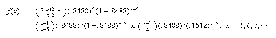
Trees are checked until 5 with
 ladybugs are found. Let
 be the total number of trees checked. Find the probability function,
 .
.
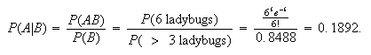
Find the probability a tree with
 ladybugs on it has exactly 6.
On 2 trees there are a total of
 ladybugs. Find the probability that
 of these are on the first of these 2 trees.
Solution:
If the ladybugs are randomly scattered the most suitable model is the Poisson
distribution with
 and
and
 (i.e. any tree has a ``volume" of 1 unit), so
 and
and
Using the binomial distribution where ``success'' means
 ladybugs on a tree, we have
 and
and
Using the negative binomial distribution, we need the number of successes,
 ,
to be 5, and the number of failures to be
,
to be 5, and the number of failures to be
 .
Then
.
Then
This is conditional probability. Let
 = { 6 ladybugs} and
 = {
= {
 ladybugs }. Then
Again we need to use conditional probability.
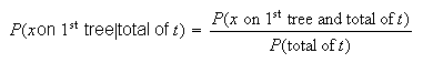
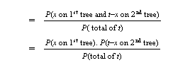 Use the Poisson distribution to calculate each, with
 in the denominator since there are 2 trees.
Caution: Don't forget to give the range of
 .
If the total is
.
If the total is
 ,
there couldn't be more than
,
there couldn't be more than
 ladybugs on the
 tree.
tree.
Exercise: The answer to (e) is a binomial probability
function. Can you reach this answer by general reasoning rather than using
conditional probability to derive it?
Problems:
In a Poisson process the average number of occurrences is
 per minute. Independent 1 minute intervals are observed until the first minute
with no occurrences is found. Let
per minute. Independent 1 minute intervals are observed until the first minute
with no occurrences is found. Let
 be the number of 1 minute intervals required, including the last one. Find the
probability function,
be the number of 1 minute intervals required, including the last one. Find the
probability function,
 .
.
Calls arrive at a telephone distress centre during the evening according to the conditions for a Poisson process. On average there are 1.25 calls per hour.
Find the probability there are no calls during a 3 hour shift.
Give an expression for the probability a person who starts working at this
centre will have the first shift with no calls on the
15 shift.
A person works one hundred 3 hour evening shifts during the year. Give an expression for the probability there are no calls on at least 4 of these 100 shifts. Calculate a numerical answer using a Poisson approximation.
| Name | Probability Function | ||
| Discrete Uniform |  |
= |  |
| Hypergeometric |  |
= |  |
| Binomial |  |
= | 
|
| Negative Binomial |  |
= |  |
| Geometric |  |
= |  |
| Poisson |  |
= |  |
 Software
The
 software system is a powerful tool for handling probability distributions and
data concerning random variables. The following short notes describe basic
features of
software system is a powerful tool for handling probability distributions and
data concerning random variables. The following short notes describe basic
features of
 ;
further information and links to other resources are available on the course
web page. Unix and Windows versions of
;
further information and links to other resources are available on the course
web page. Unix and Windows versions of
 are available on Math Faculty undergraduate servers, and free copies can be
downloaded from the web.
are available on Math Faculty undergraduate servers, and free copies can be
downloaded from the web.
You should make yourself familiar with
 ,
since some problems (and most applications of probability) require
computations or graphics which are not feasible by hand.
,
since some problems (and most applications of probability) require
computations or graphics which are not feasible by hand.
Some R Basics
R is a statistical software system that has excellent numerical,
graphical and statistical capabilities. There are Unix and Windows
versions. These notes are a very brief introduction to a few of the
features of R. Web resources have much more information. Links can
be found on the Stat 230 web page. You can also download a Unix or
Windows version of R for free.
1.PRELIMINARIES
R is invoked on Math Unix machines by typing R. The R prompt
is >. R objects include variables, functions, vectors, arrays, lists and
other items. To see online documentation about something, we use the help
function. For example, to see documentation on the function mean(), type
help(mean). In some cases help.search() is helpful.
The assignment symbol is <- : for example,
x<- 15 assigns the value 15 to variable x.
To quit an R session, type q()
2.VECTORS
Vectors can consist of numbers or other symbols; we will consider only
numbers here. Vectors are defined using c(): for example,
x<- c(1,3,5,7,9)
defines a vector of length 5 with the elements given. Vectors and other
classes of objects possess certain attributes. For example, typing
length(x) will give the length of the vector x. Vectors are a convenient
way to store values of a function (e.g. a probability function or a c.d.f)
or values of a random variable that have been recorded in some experiment
or process.
3.ARITHMETIC
The following R commands and responses should explain arithmetic
operations.
> 7+3
[1] 10
> 7*3
[1] 21
> 7/3
[1] 2.333333
> 2^3
[1] 8
4.SOME FUNCTIONS
Functions of many types exist in R. Many operate on vectors in a
transparent way, as do arithmetic operations. (For example, if x and y
are vectors then x+y adds the vectors element-wise; thus x and y must
be the same length.) Some examples, with comments, follow.
> x<- c(1,3,5,7,9) # Define a vector x
> x # Display x
[1] 1 3 5 7 9
> y<- seq(1,2,.25) #A useful function for defining a vector whose
elements are an arithmetic progression
> y
[1] 1.00 1.25 1.50 1.75 2.00
> y[2] # Display the second element of vector y
[1] 1.25
> y[c(2,3)] # Display the vector consisting of the second and
third elements of vector y.
[1] 1.25 1.50
> mean(x) #Computes the mean of the elements of vector x
[1] 5
> summary(x) # A useful function which summarizes features of
a vector x
Min. 1st Qu. Median Mean 3rd Qu. Max.
1 3 5 5 7 9
> var(x) # Computes the (sample) variance of the elements of x
[1] 10
> exp(1) # The exponential function
[1] 2.718282
> exp(y)
[1] 2.718282 3.490343 4.481689 5.754603 7.389056
> round(exp(y),2) # round(y,n) rounds the elements of vector y to
n decimals
[1] 2.72 3.49 4.48 5.75 7.39
> x+2*y
[1] 3.0 5.5 8.0 10.5 13.0
5. GRAPHS
To open a graphics window in Unix, type x11(). Note that in R, a graphics
window opens automatically when a graphical function is used.
There are various plotting and graphical functions. Two useful ones
are
plot(x,y) # Gives a scatterplot of x versus y; thus x and y must
be vectors of the same length.
hist(x) # Creates a frequency histogram based on the values in
the vector x. To get a relative frequency histogram
(areas of rectangles sum to one) use hist(x,prob=T).
Graphs can be tailored with respect to axis labels, titles, numbers of
plots to a page etc. Type help(plot), help(hist) or help(par) for some
information.
To save/print a graph in R using UNIX, you generate the graph you would
like to save/print in R using a graphing function like plot() and type:
dev.print(device,file="filename")
where device is the device you would like to save the graph to (i.e. x11)
and filename is the name of the file that you would like the graph saved
to. To look at a list of the different graphics devices you can save to,
type help(Devices).
To save/print a graph in R using Windows, you can do one of two things.
a) You can go to the File menu and save the graph using one of several
formats (i.e. postscript, jpeg, etc.). It can then be printed. You
may also copy the graph to the clipboard using one of the formats
and then paste to an editor, such as MS Word. Note that the graph
can be printed directly to a printer using this option as well.
b) You can right click on the graph. This gives you a choice of copying
the graph and then pasting to an editor, such as MS Word, or saving
the graph as a metafile or bitmap. You may also print directly to a
printer using this option as well.
6.DISTRIBUTIONS
There are functions which compute values of probability or probability
density functions, cumulative distribution functions, and quantiles for
various distributions. It is also possible to generate (pseudo) random
samples from these distributions. Some examples follow for Binomial and
Poisson distributions. For other distribution information, type
help(rhyper), help(rnbinom) and so on. Note that R does not have any
function specifically designed to generate random samples from a discrete
uniform distribution (although there is one for a continous uniform
distribution). To generate n random samples from a discrete UNIF(a,b), use
sample(a:b,n,replace=T).
> y<- rbinom(10,100,0.25) # Generate 10 random values from the Binomial
distribution Bi(100,0.25). The values are
stored in the vector y.
> y # Display the values
[1] 24 24 26 18 29 29 33 28 28 28
> pbinom(3,10,0.5) # Compute P(Y<=3) for a Bi(10,0.5) random variable.
[1] 0.171875
> qbinom(.95,10,0.5) # Find the .95 quantile (95th percentile) for
[1] 8 Bi(10,0.5).
> z<- rpois(10,10) # Generate 10 random values from the Poisson
distribution Poisson(10). The values are stored in the
vector z.
> z # Display the values
[1] 6 5 12 10 9 7 9 12 5 9
> ppois(3,10) # Compute P(Y<=3) for a Poisson(10) random variable.
[1] 0.01033605
> qpois(.95,10) # Find the .95 quantile (95th percentile) for
[1] 15 Poisson(10).
To illustrate how to plot the probability function for a random variable,
a Bi(10,0.5) random variable is used.
# Assign all possible values of the random variable, X ~ Bi(10,0.5)
x <- seq(0,10,by=1)
# Determine the value of the probability function for possible values of X
x.pf <- dbinom(x,10,0.5)
# Plot the probability function
barplot(x.pf,xlab="X",ylab="Probability Function",
names.arg=c("0","1","2","3","4","5","6","7","8","9","10"))
Suppose that the probability
 a person born in 1950 lives at least to certain ages
 is as given in the table below.
 : : |
30 | 50 | 70 | 80 | 90 | |
| Females | .980 | .955 | .910 | .595 | .240 | |
| Males | .960 | .920 | .680 | .375 | .095 |
If a female lives to age 50, what is the probability she lives to age 80? To age 90? What are the corresponding probabilities for males?
If 51% of persons born in 1950 were male, find the fraction of the total population (males and females) that will live to age 90.
Let
 be a non-negative discrete random variable with cumulative distribution
function
be a non-negative discrete random variable with cumulative distribution
function
Find the probability function of
 .
.
Find the probability of the event
 ;
the event
;
the event
 .
.
Two balls are drawn at random from a box containing ten balls numbered
 .
Let random variable
.
Let random variable
 be the larger of the numbers on the two balls and random variable
 be their total.
Tabulate the p.f. of
 and of
 if the sampling is without replacement.
Repeat (a) if the sampling is with replacement.
Let
 have a geometric distribution with
 .
Find the probability function of
.
Find the probability function of
 ,
the remainder when
,
the remainder when
 is divided by 4.
Todd decides to keep buying a lottery ticket each week until he has 4 winners (of some prize). Suppose 30% of the tickets win some prize. Find the probability he will have to buy 10 tickets.
A coffee chain claims that you have a 1 in 9 chance of winning a prize on their ``roll up the edge" promotion, where you roll up the edge of your paper cup to see if you win. If so, what is the probability you have no winners in a one week period where you bought 15 cups of coffee?
Over the last week of a month long promotion you and your friends bought 60 cups of coffee, but there was only 1 winner. Find the probability that there would be this few (i.e. 1 or 0) winners. What might you conclude?
An oil company runs a contest in which there are 500,000 tickets; a motorist receives one ticket with each fill-up of gasoline, and 500 of the tickets are winners.
If a motorist has ten fill-ups during the contest, what is the probability that he or she wins at least one prize?
If a particular gas bar distributes 2,000 tickets during the contest, what is the probability that there is at least one winner among the gas bar's customers?
Jury selection. During jury selection a large number of people are asked to be present, then persons are selected one by one in a random order until the required number of jurors has been chosen. Because the prosecution and defense teams can each reject a certain number of persons, and because some individuals may be exempted by the judge, the total number of persons selected before a full jury is found can be quite large.
Suppose that you are one of 150 persons asked to be present for the selection of a jury. If it is necessary to select 40 persons in order to form the jury, what is the probability you are chosen?
In a recent trial the numbers of men and women present for jury selection were
74 and 76. Let
 be the number of men picked for a jury of 12 persons. Give an expression for
 ,
assuming that men and women are equally likely to be picked.
,
assuming that men and women are equally likely to be picked.
For the trial in part (b), the number of men selected turned out to be two.
Find
 .
What might you conclude from this?
.
What might you conclude from this?
A waste disposal company averages 6.5 spills of toxic waste per month. Assume spills occur randomly at a uniform rate, and independently of each other, with a negligible chance of 2 or more occurring at the same time. Find the probability there are 4 or more spills in a 2 month period.
Coliform bacteria are distributed randomly and uniformly throughout river water at the average concentration of one per twenty cubic centimetres of water.
What is the probability of finding exactly two coliform bacteria in a 10 cubic centimetre sample of the river water?
What is the probability of finding at least one coliform bacterium in a 1 cubic centimetre sample of the river water?
In testing for the concentration (average number per unit volume) of bacteria
it is possible to determine cheaply whether a sample has any
(i.e. 1 or more) bacteria present or not. Suppose the average concentration of
bacteria in a body of water is
 per cubic centimetre. If 10 independent water samples of 10 c.c. each are
tested, let the random variable
per cubic centimetre. If 10 independent water samples of 10 c.c. each are
tested, let the random variable
 be the number of samples with no bacteria. Find
 .
.
Suppose that of 10 samples, 3 had no bacteria. Find an estimate for the value
of
 .
.
In a group of policy holders for house insurance, the average number of claims
per 100 policies per year is
 .
The number of claims for an individual policy holder is assumed to follow a
Poisson distribution.
.
The number of claims for an individual policy holder is assumed to follow a
Poisson distribution.
In a given year, what is the probability an individual policy holder has at least one claim?
In a group of 20 policy holders, what is the probability there are no claims in a given year? What is the probability there are two or more claims?
Assume power failures occur independently of each other at a uniform rate through the months of the year, with little chance of 2 or more occurring simultaneously. Suppose that 80% of months have no power failures.
Seven months are picked at random. What is the probability that 5 of these months have no power failures?
Months are picked at random until 5 months without power failures have been found. What is the probability that 7 months will have to be picked?
What is the probability a month has more than one power failure?
Let
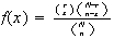 ,
and keep
,
and keep
 fixed. (e.g. If
 doubles then
 also doubles.) Prove that
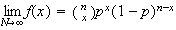 .
.
What part of the chapter is this related to?
Spruce budworms are distributed through a forest according to a Poisson
process so that the average is
 per hectare.
Give an expression for the probability that at least 1 of
 one hectare plots contains at least
 spruce budworms.
Discuss briefly which assumption(s) for a Poisson process may not be well satisfied in this situation.
A person working in telephone sales has a 20% chance of making a sale on each call, with calls being independent. Assume calls are made at a uniform rate, with the numbers made in non-overlapping periods being independent. On average there are 20 calls made per hour.
Find the probability there are 2 sales in 5 calls.
Find the probability exactly 8 calls are needed to make 2 sales.
If 8 calls were needed to make 2 sales, what is the probability there was 1 sale in the first 3 of these calls?
Find the probability of 3 calls being made in a 15 minute period.
A bin at a hardware store contains 35 forty watt lightbulbs and 70 sixty watt
bulbs. A customer wants to buy 8 sixty watt bulbs, and withdraws bulbs without
replacement until these 8 bulbs have been found. Let
 be the number of 40 watt bulbs drawn from the bin. Find the probability
function,
be the number of 40 watt bulbs drawn from the bin. Find the probability
function,
 .
.
During rush hour the number of cars passing through a particular intersection has a Poisson distribution with an average of 540 per hour.
Find the probability there are 11 cars in a 30 second interval and the probability there are 11 or more cars.
Find the probability that when 20 disjoint 30 second intervals are studied, exactly 2 of them had 11 cars.
We want to find 12 intervals having 11 cars in 30 seconds.
Give an expression for the probability 1400 30 second intervals have to be observed to find the 12 having the desired traffic flow.
Use an approximation which involves the Poisson distribution to evaluate this probability and justify why this approximation is suitable.
Bubbles are distributed in sheets of glass, as a Poisson process, at an
intensity of 1.2 bubbles per square metre. Let
 be the number of sheets of glass, in a shipment of
 sheets, which have no bubbles. Each sheet is
0.8m
sheets, which have no bubbles. Each sheet is
0.8m .
Give the probability function of
.
Give the probability function of
 .
.
The glass manufacturer wants to have at least 50% of the sheets of glass with
no bubbles. How small will the intensity
 need to be to achieve this?
Random variable
 takes values 1,2,3,4,5 and has c.d.f.
 |
0 | 1 | 2 | 3 | 4 | 5 |
 |
0 | .1 |
.2 | .5 |
 |
 |
Find
 and
and
 .
Draw a histogram of
.
Draw a histogram of
 .
.
Let random variable
 have a geometric distribution
 for
for
 .
.
Find an expression for
 ,
and show that
,
and show that
 for all non-negative integers
 ,
,
 .
.
What is the most probable value of
 ?
?
Find the probability that
 is divisible by 3.
Find the probability function of random variable
 ,
the remainder when
,
the remainder when
 is divided by 3.
Polls and Surveys. Polls or surveys in which people are
selected and their opinions or other characteristics are determined are very
widely used. For example, in a survey on cigarette use among teenage girls, we
might select a random sample of
 girls from the population in question, and determine the number
 who are regular smokers. If
 is the fraction of girls who smoke, then
 .
Since
.
Since
 is unknown (that is why we do the survey) we then estimate it as
 .
(In probability and statistics a ``hat" is used to denote an estimate of a
model parameter based on data.) The binomial distribution can be used to study
how ``good" such estimates are, as follows
.
(In probability and statistics a ``hat" is used to denote an estimate of a
model parameter based on data.) The binomial distribution can be used to study
how ``good" such estimates are, as follows
Suppose
 and
and
 .
Find the probability
.
Find the probability
 .
Many surveys try to get an estimate
.
Many surveys try to get an estimate
 which is within 3% (.03) of
 with high probability. What do you conclude here?
Repeat the calculation in (a) if
 and
and
 .
What do you conclude?
.
What do you conclude?
If
 instead of .3, find
 when
when
 and 1000.
Your employer asks you to design a survey to estimate the fraction
 of persons age 25-34 who download music via the internet. The objective is to
get an estimate accurate to within 3%, with probability close to .95. What
size of sample
of persons age 25-34 who download music via the internet. The objective is to
get an estimate accurate to within 3%, with probability close to .95. What
size of sample
 would you recommend?
Telephone surveys. In some ``random digit dialing" surveys, a computer phones randomly selected telephone numbers. However, not all numbers are ``active" (belong to a telephone account) and they may belong to businesses as well as to individual or residences.
Suppose that for a given large set of telephone numbers, 57% are active residential or individual numbers. We will call these ``personal" numbers.
Suppose that we wish to interview (over the phone) 1000 persons in a survey.
Suppose that the probability a call to a personal number is answered is .8,
and that the probability the person answering agrees to be interviewed is .7.
Give the probability distribution for
 ,
the number of calls needed to obtain 1000 interviews.
,
the number of calls needed to obtain 1000 interviews.
Use R software to find
 for the values
 .
.
Suppose instead that 3200 randomly selected numbers were dialed. Give the
probability distribution for
 ,
the number of interviews obtained, and find
,
the number of interviews obtained, and find
 .
.
(Note: The R functions pnbinom and pbinom give negative binomial and binomial probabilities, respectively.)