7. Expectation, Averages, Variability
Summarizing Data on Random Variables
When we return midterm tests, someone almost always asks what the average was.
While we could list out all marks to give a picture of how students performed,
this would be tedious. It would also give more detail than could be
immediately digested. If we summarize the results by telling a class the
average mark, students immediately get a sense of how well the class
performed. For this reason, "summary statistics" are often more helpful than
giving full details of every outcome.
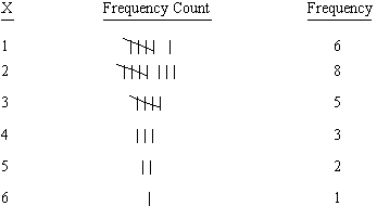
To illustrate some of the ideas involved, suppose we were to observe cars
crossing a toll bridge, and record the number,
 ,
of people in each car. Suppose in a small study data on 25 cars were
collected. We could list out all 25 numbers observed, but a more helpful way
of presenting the data would be in terms of the frequency
distribution below, which gives the number of times (the
``frequency'') each value of
,
of people in each car. Suppose in a small study data on 25 cars were
collected. We could list out all 25 numbers observed, but a more helpful way
of presenting the data would be in terms of the frequency
distribution below, which gives the number of times (the
``frequency'') each value of
 occurred.
We could also draw a frequency histogram of these
frequencies:
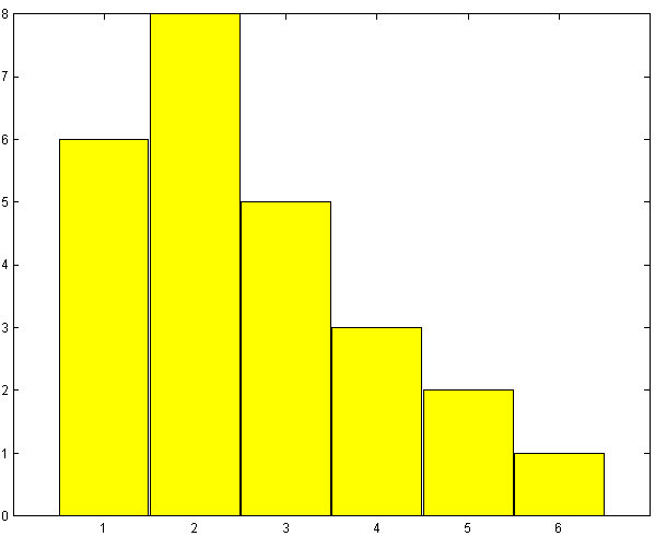
Frequency distributions or histograms are good summaries of data because they
show the variability in the observed outcomes very clearly. Sometimes,
however, we might prefer a single-number summary. The most common such summary
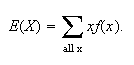
is the average, or arithmetic mean of the outcomes. The mean of
 outcomes
 for a random variable
 is
is
 ,
and is denoted by
,
and is denoted by
 .
The arithmetic mean for the example above can be calculated as
.
The arithmetic mean for the example above can be calculated as
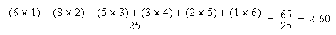 That is, there was an average of 2.6 persons per car. A set of observed
outcomes
That is, there was an average of 2.6 persons per car. A set of observed
outcomes
 for a random variable
 is termed a sample in probability and statistics. To reflect
the fact that this is the average for a particular sample, we refer to it as
the sample mean. Unless somebody deliberately "cooked" the
study, we would not expect to get precisely the same sample mean if we
repeated it another time. Note also that
is termed a sample in probability and statistics. To reflect
the fact that this is the average for a particular sample, we refer to it as
the sample mean. Unless somebody deliberately "cooked" the
study, we would not expect to get precisely the same sample mean if we
repeated it another time. Note also that
 is not in general an integer, even though
 is.
is.
Two other common summary
statistics are the median and mode.
Definition
The median of a sample is a value such that half the results
are below it and half above it, when the results are arranged in numerical
order.
If these 25 results were written in order, the
 outcome would be a 2. So the median is 2. By convention, we go half way
between the middle two values if there are an even number of observations.
outcome would be a 2. So the median is 2. By convention, we go half way
between the middle two values if there are an even number of observations.
Definition
The mode of the sample is the value which occurs most often.
In this case the mode is 2. There is no guarantee there will be only a single
mode.
Expectation of a Random Variable
The statistics in the preceding section summarize features of a sample of
observed
 -values.
The same idea can be used to summarize the probability distribution of a
random variable
-values.
The same idea can be used to summarize the probability distribution of a
random variable
 .
To illustrate, consider the previous example, where
.
To illustrate, consider the previous example, where
 is the number of persons in a randomly selected car crossing a toll bridge.
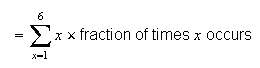
Note that we can re-arrange the expression used to calculate
 for the sample,
as
for the sample,
as
 Now suppose we know that the probability function of
 is given by
 |
1 |
2 |
3 |
4 |
5 |
6 |
 |
.30 |
.25 |
.20 |
.15 |
.09 |
.01 |
Using the relative frequency ``definition'' of
probability, if we observed a very large number of cars, the fraction (or
relative frequency) of times
 would be .30, for
 ,
this proportion would be .25, etc. So, in theory,
(according to the probability model) we would expect the mean to be
,
this proportion would be .25, etc. So, in theory,
(according to the probability model) we would expect the mean to be
 if we observed an infinite number of cars. This ``theoretical'' mean is
usually denoted by
if we observed an infinite number of cars. This ``theoretical'' mean is
usually denoted by
 or
or
 ,
and requires us to know the distribution of
,
and requires us to know the distribution of
 .
With this background we make the following mathematical
definition.
.
With this background we make the following mathematical
definition.
The expectation of
 is also often denoted by the Greek letter
 .
The expectation of
.
The expectation of
 can be thought of physically as the average of the
 -values
that would occur in an infinite series of repetitions of the process where
-values
that would occur in an infinite series of repetitions of the process where
 is defined. This value not only describes one aspect of a probability
distribution, but is also very important in certain types of applications. For
example, if you are playing a casino game in which
is defined. This value not only describes one aspect of a probability
distribution, but is also very important in certain types of applications. For
example, if you are playing a casino game in which
 represents the amount you win in a single play, then
 represents your average winnings (or losses!) per play.
Sometimes we may not be interested in the average value of
 itself, but in some function of
 .
Consider the toll bridge example once again, and suppose there is a toll which
depends on the number of car occupants. For example, a toll of $1 per car plus
25 cents per occupant would produce an average toll for the 25 cars in the
study of Section 7.1 equal to
.
Consider the toll bridge example once again, and suppose there is a toll which
depends on the number of car occupants. For example, a toll of $1 per car plus
25 cents per occupant would produce an average toll for the 25 cars in the
study of Section 7.1 equal to
 If
If
 has the theoretical probability function
 given above, then the average value of this $(.25X + 1) toll would be defined
in the same way, as,
given above, then the average value of this $(.25X + 1) toll would be defined
in the same way, as,

We call this the expectation of
 and write
 .
.
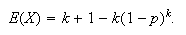
As a further illustration, suppose a toll designed to encourage car pooling
charged
 if there were
 people in the car. This scheme would yield an average toll, in theory, of

that
is, is the ``expectation'' of
 .
.
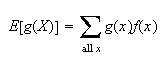
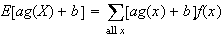
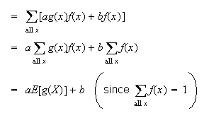
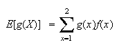
With this as background, we can now make a formal definition.
Notes:
-
You can interpret
![$E[g(X)]$](graphics/noteschap7__59.png) as the average value of
as the average value of
 in an infinite series of repetitions of the process where
 is defined.
-
 is also known as the ``expected value'' of
 .
This name is somewhat misleading since the average value of
.
This name is somewhat misleading since the average value of
 may be a value which
 never takes - hence unexpected!
-
The case where
 reduces to our earlier definition of
 .
.
-
Confusion sometimes arises because we have two notations for the mean of a
probability distribution:
 and
and
 mean the same thing. There is nothing wrong with this.
-
When calculating expectations, look at your answer to be sure it makes sense.
If
 takes values from 1 to 10, you should know you've made an error if you get
 or
or
 .
In physical terms,
.
In physical terms,
 is the balance point for the histogram of
 .
.
Let us note a couple of mathematical properties of expectation that can help
to simplify calculations.
Properties of Expectation:
If your linear algebra is good, it may help if you think of
 as being a linear operator. Otherwise you'll have to remember these and
subsequent properties.
as being a linear operator. Otherwise you'll have to remember these and
subsequent properties.
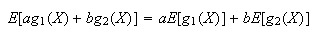
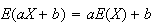
-
For constants
 and
and
 ,
,
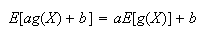
Proof:
-
For constants
 and
and
 and functions
 and
and
 ,
it is also easy to show
,
it is also easy to show
 Don't let expectation intimidate you. Much of it is common sense. For example,
property 1 says
Don't let expectation intimidate you. Much of it is common sense. For example,
property 1 says
 if we let
 and
and
 .
The expectation of a constant
.
The expectation of a constant
 is of course equal to
 .
It also says
.
It also says
 if we let
 ,
,
 ,
and
,
and
 .
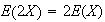
This is obvious also. Note, however, that for
.
This is obvious also. Note, however, that for
 a nonlinear function, it is not true that
![$E[g(X)]=g(E(X))$](graphics/noteschap7__96.png) ;
this is a common mistake. (Check this for the example above when
;
this is a common mistake. (Check this for the example above when
 .)
.)
Some Applications of Expectation
Because expectation is an average value, it is frequently used in problems
where costs or profits are connected with the outcomes of a random variable
 .
It is also used a lot as a summary statistic for probability distributions;
for example, one often hears about the expected life (expectation of lifetime)
for a person or the expected return on an investment.
.
It is also used a lot as a summary statistic for probability distributions;
for example, one often hears about the expected life (expectation of lifetime)
for a person or the expected return on an investment.
The following are examples.
Example: Expected Winnings in a Lottery
A small lottery sells 1000 tickets numbered
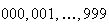 ;
the tickets cost $10 each. When all the tickets have been sold the draw takes
place: this consists of a simple ticket from 000 to 999 being chosen at
random. For ticket holders the prize structure is as follows:
;
the tickets cost $10 each. When all the tickets have been sold the draw takes
place: this consists of a simple ticket from 000 to 999 being chosen at
random. For ticket holders the prize structure is as follows:
-
Your ticket is drawn - win $5000.
-
Your ticket has the same first two number as the winning ticket, but the third
is different - win $100.
-
Your ticket has the same first number as the winning ticket, but the second
number is different - win $10.
-
All other cases - win nothing.
Let the random variable
 represent the winnings from a given ticket. Find
 .
.
Solution: The possible values for
 are 0, 10, 100, 5000 (dollars). First, we need to find the probability
function for
are 0, 10, 100, 5000 (dollars). First, we need to find the probability
function for
 .
We find (make sure you can do this) that
.
We find (make sure you can do this) that
 has values

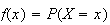
The expected winnings are thus the expectation of
 ,
or
,
or
 Thus, the gross expected winnings per ticket are $6.80. However, since a
ticket costs $10 your expected net winnings are negative, -$3.20 (i.e. an
expected loss of $3.20).
Thus, the gross expected winnings per ticket are $6.80. However, since a
ticket costs $10 your expected net winnings are negative, -$3.20 (i.e. an
expected loss of $3.20).
Remark: For any lottery or game of chance the expected net
winnings per play is a key value. A fair game is one for which this value is
0. Needless to say, casino games and lotteries are never fair: the net
winnings for a player are
negative.
Remark: The random variable associated with a given
problem may be defined in different ways but the expected winnings will remain
the same. For example, instead of defining
 as the amount won we could have defined
 as follows:
 |
|
all 3 digits of number match winning ticket |
 |
|
1st 2 digits (only) match |
 |
|
1st digit (but not the 2nd) match |
 |
|
1st digit does not match |
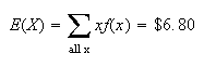
Now, we would define the function
 as the winnings when the outcome
 occurs. Thus,

The expected winnings are then
 the same as before.
Example: Diagnostic Medical Tests
Often there are cheaper, less accurate tests for diagnosing the presence of
some conditions in a person, along with more expensive, accurate tests.
Suppose we have two cheap tests and one expensive test, with the following
characteristics. All three tests are positive if a person has the condition
(there are no "false negatives"), but the cheap tests give "false positives".
Let a person be chosen at random, and let
 = {person has the condition}. The three tests are
| Test 1: |
|
 (positive test
 = .05; test costs $5.00
 |
| Test 2: |
|
 (positive test
 = .03; test costs $8.00
 |
| Test 3: |
|
 (positive test
 = 0; test costs $40.00
 |
We want to check a large number of people for the condition, and have to
choose among three testing strategies:
-
Use Test 1, followed by Test 3 if Test 1 is positive.
-
Use Test 2, followed by Test 3 if Test 2 is positive.
-
Use Test 3.
Determine the expected cost per person under each of strategies (i), (ii) and
(iii). We will then choose the strategy with the lowest expected cost. It is
known that about .001 of the population have the condition (i.e.
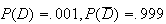 ).
).
Solution: Define the random variable
 as follows (for a random person who is tested):
 |
|
if the initial test is negative |
 |
|
if the initial test is positive |
Also let
 be the total cost of testing the person. The expected cost per person is then
The probability function
 for
for
 and function
 differ for strategies (i), (ii) and (iii). Consider for example strategy (i).
Then
differ for strategies (i), (ii) and (iii). Consider for example strategy (i).
Then
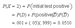 The rest if the probabilities, associated values of
 and
and
![$E[g(X)]$](graphics/noteschap7__140.png) are obtained below.
are obtained below.
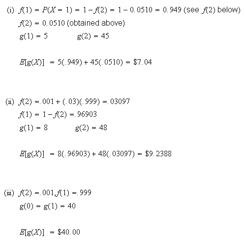
Thus, its cheapest to use strategy
(i).
Problem:
-
A lottery has tickets numbered 000 to 999 which are sold for $1 each. One
ticket is selected at random and a prize of $200 is given to any person whose
ticket number is a permutation of the selected ticket number. All 1000 tickets
are sold. What is the expected profit or loss to the organization running the
lottery?
Means and Variances of Distributions
Its useful to know the means,
 of probability models derived in Chapter
6.
of probability models derived in Chapter
6.
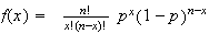
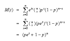
Example: (Mean of binomial distribution)
Let
 .
Find
.
Find
 .
.
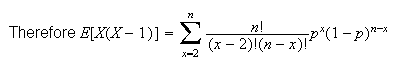
Solution:
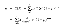
When
 the value of the expression is 0. We can therefore begin our sum at
 .
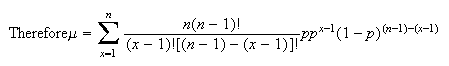
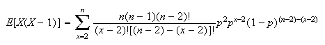
Provided
.
Provided
 ,
we can expand
,
we can expand
 as
as
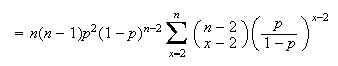
 (so it is important to eliminate the term when
 ).
).
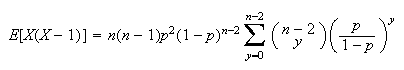
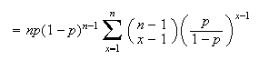 Let
Let
 in the sum, to get
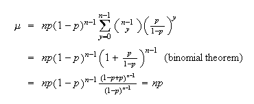
Exercise: Does this result make sense? If you try something
100 times and there is a 20% chance of success each time, how many successes
do you expect to get, on
average?
Example: (Mean of the Poisson
distribution)
Let
 have a Poisson distribution where
 is the average rate of occurrence and the time interval is of length
 .
Find
.
Find
 .
.
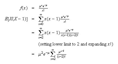
Solution:
The probability function of
 is
is
 .
Then
.
Then
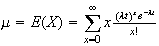 .
.
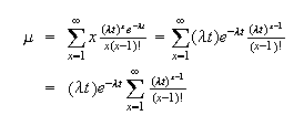
As in the binomial example, we can eliminate the term when
 and expand
 as
as
 for
for
 .
.
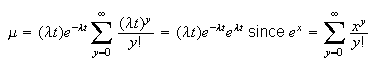
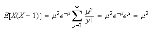
 Let
Let
 in the sum.
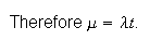 Note that we used the symbol
 earlier in connection with the Poisson model; this was because we knew (but
couldn't show until now) that
earlier in connection with the Poisson model; this was because we knew (but
couldn't show until now) that
 .
.
Exercise: These techniques can also be used to work out the
mean for the hypergeometric or negative binomial distributions. Looking back
at how we proved that
 shows the same method of summation used to find
 .
However, in Chapter 8 we will give a simpler method of finding the means of
these distributions, which are
.
However, in Chapter 8 we will give a simpler method of finding the means of
these distributions, which are
 (hypergeometric) and
 (negative binomial).
Variability:
While an average is a useful summary of a set of observations, or of a
probability distribution, it omits another important piece of information,
namely the amount of variability. For example, it would be possible for car
doors to be the right width, on average, and still have no doors fit properly.
In the case of fitting car doors, we would also want the door widths to all be
close to this correct average. We give a way of measuring the amount of
variability next. You might think we could use the average difference between
 and
and
 to indicate the amount of variation. In terms of expectation, this would be
 .
However,
.
However,
 (since
 is a constant) = 0. We soon realize that to measure variability we need a
function that is the same sign for
is a constant) = 0. We soon realize that to measure variability we need a
function that is the same sign for
 and for
 .
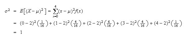
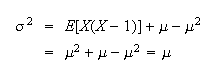
We now define
.
We now define
In words, the variance is the
average square of the distance from the mean. This turns out to be a very
useful measure of the variability of
 .
.
Example: Let
 be the number of heads when a fair coin is tossed 4 times. Then
 so
so
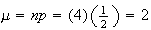 .
Without doing any calculations we know
.
Without doing any calculations we know
 because
 is always between 0 and 4. Hence it can never be further away from
 than 2. This makes the average square of the distance from
 at most 4. The values of
 are
are
 |
0 |
1 |
2 |
3 |
4 |
since
 |
= |
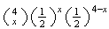 |
 |
1/16 |
4/16 |
6/16 |
4/16 |
1/16 |
|
= |
 |
The value of
 (i.e.
(i.e.
 )
is easily found here:
)
is easily found here:
If we keep track of units of
measurement the variance will be in peculiar units; e.g. if
 is the number of heads in 4 tosses of a coin,
 is in units of
heads
is in units of
heads !
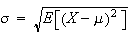
We can regain the original units by taking (positive)
!
We can regain the original units by taking (positive)
 .
This is called the standard deviation of
.
This is called the standard deviation of
 ,
and is denoted by
,
and is denoted by
 ,
or as
,
or as
 .
.
Definition
The standard deviation of a random variable
 is
is
Both variance and standard
deviation are commonly used to measure variability.
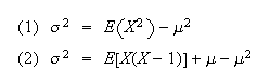
The basic definition of
variance is often awkward to use for mathematical calculation of
 ,
whereas the following two results are often useful:
,
whereas the following two results are often useful:
Proof:
-
Using properties of expectation,
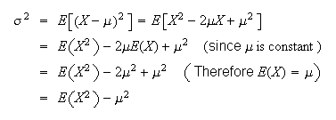
(2)

Formula (2) is most often used when there is an
 term in the denominator of
 .
Otherwise, formula (1) is generally easier to
use.
.
Otherwise, formula (1) is generally easier to
use.
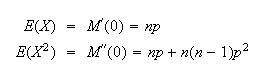
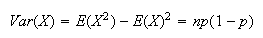
Example: (Variance of binomial distribution)
Let
 .
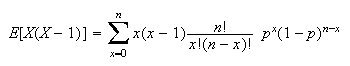
Find Var
.
Find Var

Solution:
 ,
so we'll use formula (2).
,
so we'll use formula (2).
If
 or
or
 the value of the term is 0, so we can begin summing at
 .
For
.
For
 or
or
 ,
we can expand the
,
we can expand the
 as
as
 Now re-group to fit the binomial theorem, since that was the summation
technique used to show
Now re-group to fit the binomial theorem, since that was the summation
technique used to show
 and to derive
 .
.
 Let
Let
 in the sum, giving
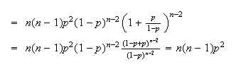 Then
Then
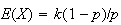
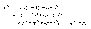 Remember that the variance of a binomial distribution is
 ,
since we'll be using it later in the
course.
,
since we'll be using it later in the
course.
Example: (Variance of Poisson distribution) Find the
variance of the Poisson distribution.
Solution:
 Let
Let
 in the sum, giving
 (that is, for the Poisson, the variance equals the
mean.)
(that is, for the Poisson, the variance equals the
mean.)
Properties of Mean and Variance
If
 and
and
 are constants and
 ,
then
,
then
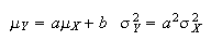
(where
 and
and
 are the mean and variance of
 and
and
 and
and
 are the mean and variance of
 ).
).
Proof:
We already showed that
 .
.
i.e.
 ,
and then
,
and then
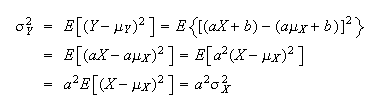
This result is to be expected. Adding a constant,
 ,
to all values of
,
to all values of
 has no effect on the amount of variability. So it makes sense that Var
 doesn't depend on the value of
 .
.
A simple way to relate to this result is to consider a random variable
 which represents a temperature in degrees Celsius (even though this is a
continuous random variable which we don't study until Chapter 9). Now let
which represents a temperature in degrees Celsius (even though this is a
continuous random variable which we don't study until Chapter 9). Now let
 be the corresponding temperature in degrees Fahrenheit. We know that
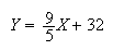 and it is clear if we think about it that
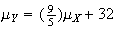 and that
 .
.
Problems:
-
An airline knows that there is a 97% chance a passenger for a certain flight
will show up, and assumes passengers arrive independently of each other.
Tickets cost $100, but if a passenger shows up and can't be carried on the
flight the airline has to refund the $100 and pay a penalty of $400 to each
such passenger. How many tickets should they sell for a plane with 120 seats
to maximize their expected ticket revenues after paying any penalty charges?
Assume ticket holders who don't show up get a full refund for their unused
ticket.
-
A typist typing at a constant speed of 60 words per minute makes a mistake in
any particular word with probability .04, independently from word to word.
Each incorrect word must be corrected; a task which takes 15 seconds per word.
-
Find the mean and variance of the time (in seconds) taken to finish a 450 word
passage.
-
Would it be less time consuming, on average, to type at 45 words per minute if
this reduces the probability of an error to .02?
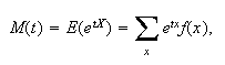
Moment Generating Functions
We have now seen two functions which characterize a distribution, the
probability function and the cumulative distribution function. There is a
third type of function, the moment generating
function, which uniquely determines a distribution. The moment
generating function is closely related to other transforms used in
mathematics, the Laplace and Fourier transforms.
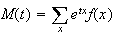
The moments of a random variable
 are the expectations of the functions
 for
for
 .
The expectation
.
The expectation
 is called
 moment of
 .
The mean
.
The mean
 is therefore the first moment,
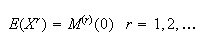
 the second and so on. It is often easy to find the moments of a probability
distribution mathematically by using the moment generating function. This
often gives easier derivations of means and variances than the direct
summation methods in the preceding section. The following theorem gives a
useful property of m.g.f.'s.
the second and so on. It is often easy to find the moments of a probability
distribution mathematically by using the moment generating function. This
often gives easier derivations of means and variances than the direct
summation methods in the preceding section. The following theorem gives a
useful property of m.g.f.'s.
Proof:
 and if the sum converges, then
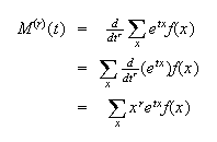
 ,
as stated.
,
as stated.
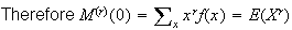
This sometimes gives a simple way to find the moments for a distribution.
Example 1.
![MATH]()


and
so
 From this we can also find
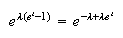
Exercise. Poisson distribution
Show that the Poisson distribution with probability function
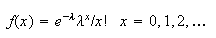 has m.g.f.
 .
Then show that
.
Then show that
 and
and
 .
.
The m.g.f. also uniquely
identifies a distribution in the sense that two different distributions cannot
have the same m.g.f. This result is often used to find the distribution of a
random variable.
The other feature of the moment generating function that is often used is that
it can be used to identify a given distribution. If two random variables have
the same moment generating function, they have the same distribution (so the
same probability function, cumulative distribution function, moments, etc.)
But in fact moment generating functions can also be used to determine that a
sequence of distributions gets closer and closer to some limiting
distribution. To show this, suppose that a sequence of probability functions
 have corresponding moment generating functions
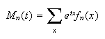 Suppose moreover that the probability functions
 converge to another probability function
 pointwise in
 as
as
 .
This is what we mean by convergence of discrete distributions. Then since
.
This is what we mean by convergence of discrete distributions. Then since
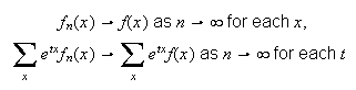 which says that
 converges to
 the moment generating function of the limiting distribution. It shouldn't be
too surprising that a very useful converse to this result also holds:
the moment generating function of the limiting distribution. It shouldn't be
too surprising that a very useful converse to this result also holds:
Suppose
 has moment generating function
 and
and
 for each
 such that
 For example we saw in Chapter 6 that a
Binomial
For example we saw in Chapter 6 that a
Binomial distribution with very large
 and very small
 is close to a Poisson distribution with parameter
 Consider the moment generating function of such a binomial random
variable
Consider the moment generating function of such a binomial random
variable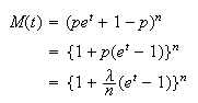 Now consider the limit of this expression as
 Since in general
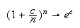 the limit of (binmgf) as
 is
is
 and this is the moment generating function of a Poisson distribution with
parameter
and this is the moment generating function of a Poisson distribution with
parameter
 This shows a little more formally than we did earlier that the
binomial
This shows a little more formally than we did earlier that the
binomial distribution with
 approaches the
Poisson(
approaches the
Poisson( )
distribution as
)
distribution as

Problems on Chapter 7
-
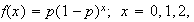
Let
 have probability function
 Find the mean and variance for
 .
.
-
A game is played where a fair coin is tossed until the first tail occurs. The
probability
 tosses will be needed is
 .
You win
.
You win
 if
if
 tosses are needed for
 but lose $256 if
 .
Determine your expected winnings.
.
Determine your expected winnings.
-
Diagnostic tests. Consider diagnostic tests like those discussed above in the
example of Section 7.3 and in Problem 15 for Chapter 4. Assume that for a
randomly selected person,
 ,
,
 ,
,
 ,
so that the inexpensive test only gives false positive, and not false
negative, results.
,
so that the inexpensive test only gives false positive, and not false
negative, results.
Suppose that this inexpensive test costs $10. If a
person tests positive then they are also given a more expensive test, costing
$100, which correctly identifies all persons with the disease. What is the
expected cost per person if a population is tested for the disease using the
inexpensive test followed, if necessary, by the expensive test?
-
Diagnostic tests II. Two percent of the population has a certain condition for
which there are two diagnostic tests. Test A, which costs $1 per person, gives
positive results for 80% of persons with the condition and for 5% of persons
without the condition. Test B, which costs $100 per person, gives positive
results for all persons with the condition and negative results for all
persons without it.
-
-
Suppose that test B is given to 150 persons, at a cost of $15,000. How many
cases of the condition would one expect to detect?
-
Suppose that 2000 persons are given test A, and then only those who test
positive are given test B. Show that the expected cost is $15,000 but that the
expected number of cases detected is much larger than in part (a).
-
The probability that a roulette wheel stops on a red number is 18/37. For each
bet on ``red'' you win the amount bet if the wheel stops on a red number, and
lose your money if it does not.
-
-
If you bet $1 on each of 10 consecutive plays, what is your expected winnings?
What is your expected winnings if you bet $10 on a single play?
-
For each of the two cases in part (a), calculate the probability that you made
a profit (that is, your ``winnings'' are positive, not negative).
-
Slot machines. Consider the slot machine discussed above in Problem 16 for
Chapter 4. Suppose that the number of each type of symbol on wheels 1, 2 and 3
is as given below:
| |
 |
Wheel |
| |
|
|
|
|
| Symbols |
|
1 |
2 |
3 |
|
Flower |
|
2 |
6 |
2 |
|
Dog |
|
4 |
3 |
3 |
|
House |
|
4 |
1 |
5 |
If all three wheels stop on a flower, you win $20 for a $1 bet. If all three
wheels stop on a dog, you win $10, and if all three stop on a house, you win
$5. Otherwise you win nothing.
Find your expected winnings per dollar spent.
-
Suppose that
 people take a blood test for a disease, where each person has probability
 of having the disease, independent of other persons. To save time and money,
blood samples from
of having the disease, independent of other persons. To save time and money,
blood samples from
 people are pooled and analyzed together. If none of the
 persons has the disease then the test will be negative, but otherwise it will
be positive. If the pooled test is positive then each of the
persons has the disease then the test will be negative, but otherwise it will
be positive. If the pooled test is positive then each of the
 persons is tested separately (so
 tests are done in that case).
-
-
A manufacturer of car radios ships them to retailers in cartons of
 radios. The profit per radio is $59.50, less shipping cost of $25 per carton,
so the profit is $
radios. The profit per radio is $59.50, less shipping cost of $25 per carton,
so the profit is $
 per carton. To promote sales by assuring high quality, the manufacturer
promises to pay the retailer
per carton. To promote sales by assuring high quality, the manufacturer
promises to pay the retailer
 if
if
 radios in the carton are defective. (The retailer is then responsible for
repairing any defective radios.) Suppose radios are produced independently and
that 5% of radios are defective. How many radios should be packed per carton
to maximize expected net profit per carton?
radios in the carton are defective. (The retailer is then responsible for
repairing any defective radios.) Suppose radios are produced independently and
that 5% of radios are defective. How many radios should be packed per carton
to maximize expected net profit per carton?
-
Let
 have a geometric distribution with probability
function
have a geometric distribution with probability
function
-
-
Calculate the m.g.f.
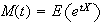 ,
where
,
where
 is a parameter.
-
Find the mean and variance of
 .
.
-
Use your result in (b) to show that if
 is the probability of ``success''
(
is the probability of ``success''
( )
in a sequence of Bernoulli trials, then the expected number of trials until
the first
)
in a sequence of Bernoulli trials, then the expected number of trials until
the first
 occurs is
 .
Explain why this is ``obvious''.
.
Explain why this is ``obvious''.
-
Analysis of Algorithms: Quicksort. Suppose we have a set
 of distinct numbers and we wish to sort them from smallest to largest. The
quicksort algorithm works as follows: When
of distinct numbers and we wish to sort them from smallest to largest. The
quicksort algorithm works as follows: When
 it just compares the numbers and puts the smallest one first. For
 it starts by choosing a random "pivot" number from the
 numbers. It then compares each of the other
 numbers with the pivot and divides them into groups
 (numbers smaller than the pivot) and
 ( numbers bigger than the pivot). It then does the same thing with
 and
and
 as it did with
 ,
and repeats this recursively until the numbers are all sorted. (Try this out
with, say
,
and repeats this recursively until the numbers are all sorted. (Try this out
with, say
 numbers to see how it works.) In computer science it is common to analyze such
algorithms by finding the expected number of comparisons (or other operations)
needed to sort a list. Thus, let
numbers to see how it works.) In computer science it is common to analyze such
algorithms by finding the expected number of comparisons (or other operations)
needed to sort a list. Thus, let

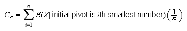
-
Show that if
 is the number of comparisons needed,
-
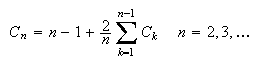
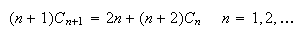
Show that
 and thus that
 satisfies the recursion (note
 )
)
-
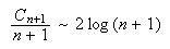
Show that
-
(Harder) Use the result of part (c) to show that for large
 ,
,
 (Note:
 means
means
 as
as
 )
This proves a result from computer science which says that for Quicksort,
)
This proves a result from computer science which says that for Quicksort,
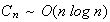 .
.
-
Find the distributions that corresponds to the following moment-generating
functions:
(a)

(b)

-
Find the moment generating function of the discrete uniform distribution
 on
on
 ;
;
 What do you get in the special case
 and in the case
 Use the moment generating function in these two cases to confirm the expected
value and the variance of
Use the moment generating function in these two cases to confirm the expected
value and the variance of

-
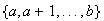
Let
 be a random variable taking values in the set
 with moments
 ,
,

-
Find the moment generating function of

-
Find the first six moments of

-
Find
-
Show that any probability distribution on
 is completely determined by its first two moments.