8. Discrete Multivariate Distributions
Basic Terminology and Techniques
Many problems involve more than a single random variable. When there are
multiple random variables associated with an experiment or process we usually
denote them as
 or as
or as
 .
For example, your final mark in a course might involve
.
For example, your final mark in a course might involve
 -- your assignment mark,
 -- your midterm test mark, and
 -- your exam mark. We need to extend the ideas introduced for single variables
to deal with multivariate problems. In this course we only consider discrete
multivariate problems, though continuous multivariate variables are also
common in daily life (e.g. consider a person's height
-- your exam mark. We need to extend the ideas introduced for single variables
to deal with multivariate problems. In this course we only consider discrete
multivariate problems, though continuous multivariate variables are also
common in daily life (e.g. consider a person's height
 and weight
 ).
).
To introduce the ideas in a simple setting, we'll first consider an example in
which there are only a few possible values of the variables. Later we'll apply
these concepts to more complex examples. The ideas themselves are simple even
though some applications can involve fairly messy algebra.
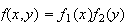
Joint Probability Functions:
First, suppose there are two r.v.'s
 and
and
 ,
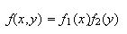
and define the function
,
and define the function
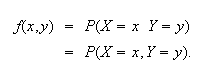
We call
 the joint probability function of
 .
In general,
.
In general,
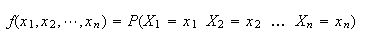 if there are
 r.v.'s
 .
.
The properties of a joint probability function are similar to those for a
single variable; for two r.v.'s we have
 for all
 and
and
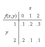
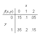
Example: Consider the following numerical example, where we
show
 in a table.
|
|
 |
 |
0 |
1 |
2 |
|
1 |
.1 |
.2 |
.3 |
 |
|
|
|
|
|
2 |
.2 |
.1 |
.1 |
for example
 and
and

We can check that
 is a proper joint probability function since
 for all 6 combinations of
 and the sum of these 6 probabilities is 1. When there are only a few values
for
and the sum of these 6 probabilities is 1. When there are only a few values
for
 and
and
 it is often easier to tabulate
 than to find a formula for it. We'll use this example below to illustrate
other definitions for multivariate distributions, but first we give a short
example where we need to find
than to find a formula for it. We'll use this example below to illustrate
other definitions for multivariate distributions, but first we give a short
example where we need to find
 .
.
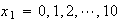
Example: Suppose a fair coin is tossed 3 times. Define the
r.v.'s
 = number of Heads and
 if
if
 occurs on the first toss. Find the joint probability function for
 .
.
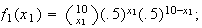
Solution: First we should note the range for
 ,
which is the set of possible values
,
which is the set of possible values
 which can occur. Clearly
 can be 0, 1, 2, or 3 and
 can be 0 or 1, but we'll see that not all 8 combinations
 are possible.
We can find
 by just writing down the sample space
 that we have used before for this process. Then simple counting gives
 as shown in the following table:
For example,
 iff the outcome is
 iff the outcome is either
 or
or
 .
.
Note that the range or joint p.f. for
 is a little awkward to write down here in formulas, so we just use the
table.
is a little awkward to write down here in formulas, so we just use the
table.
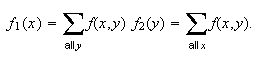
Marginal Distributions:
We may be given a joint probability function involving more variables than
we're interested in using. How can we eliminate any which are not of interest?
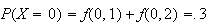
Look at the first example above. If we're only interested in
 ,
and don't care what value
,
and don't care what value
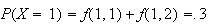
 takes, we can see that
 so
so
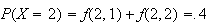
 Similarly
 and
and
The distribution of
 obtained in this way from the joint distribution is called the marginal
probability function of
obtained in this way from the joint distribution is called the marginal
probability function of
 :
:
 |
0 |
1 |
2 |
 |
.3 |
.3 |
.4 |
In the same way, if we were only interested in
 ,
we obtain
,
we obtain
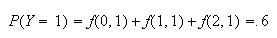 since
since
 can be 0, 1, or 2 when
 .
The marginal probability function of
.
The marginal probability function of
 would be:
 |
1 |
2 |
 |
.6 |
.4 |
Our notation for marginal probability functions is still inadequate. What is
 ?
As soon as we substitute a number for
?
As soon as we substitute a number for
 or
or
 ,
we don't know which variable we're referring to. For this reason, we generally
put a subscript on the
,
we don't know which variable we're referring to. For this reason, we generally
put a subscript on the
 to indicate whether it is the marginal probability function for the first or
second variable. So
to indicate whether it is the marginal probability function for the first or
second variable. So
 would be
 ,
while
,
while
 would be
 .
.
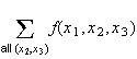
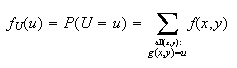
In general, to find
 we add over all values of
 where
where
 ,
and to find
,
and to find
 we add over all values of
 with
with
 .
Then
.
Then
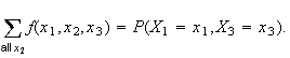
This reasoning can be extended beyond two variables. For example, with 3
variables
 ,
,
-
 would be
 and
and
-
 would be
Independent Random Variables:
For events
 and
and
 ,
we have defined
,
we have defined
 and
and
 to be independent
iff
to be independent
iff
 .
This definition can be extended to random variables
.
This definition can be extended to random variables

Definition
In general,
 are independent random variables
iff
are independent random variables
iff

In our first example
 and
and
 are not independent since
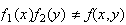 for any of the 6 combinations of
 values; e.g.,
 but
but
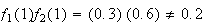 .
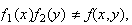
Be careful applying this definition. You can only conclude that
.
Be careful applying this definition. You can only conclude that
 and
and
 are independent after checking
all
are independent after checking
all  combinations. Even a single case where
 makes
makes
 and
and
 dependent.
Conditional Probability Functions:
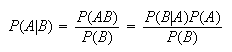
Again we can extend a definition from events to random variables. For events
 and
and
 ,
recall that
,
recall that
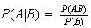 .
Since
.
Since
 ,
we make the following definition.
,
we make the following definition.
In our first example let us
find
 .
.
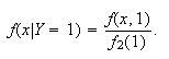 This gives:
As you would expect, marginal and conditional probability functions are
probability functions in that they are always
 and their sum is 1.
Functions of Variables:
In an example earlier, your final mark in a course might be a function of the
3 variables
 - assignment, midterm, and exam
marks Note_1 . Indeed, we often
encounter problems where we need to find the probability distribution of a
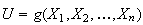
function of two or more r.v.'s. The most general method for finding the
probability function for some function of random variables
- assignment, midterm, and exam
marks Note_1 . Indeed, we often
encounter problems where we need to find the probability distribution of a
function of two or more r.v.'s. The most general method for finding the
probability function for some function of random variables
 and
and
 involves looking at every combination
 to see what value the function takes. For example, if we let
 in our example, the possible values of
 are seen by looking at the value of
 for each
 in the range of
 .
.
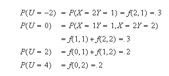
The probability function of
 is thus
 |
-2 |
0 |
2 |
4 |
 |
.3 |
.3 |
.2 |
.2 |
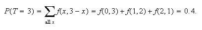
For some functions it is possible to approach the problem more systematically.
One of the most common functions of this type is the total. Let
 .
This gives:
.
This gives:
Then
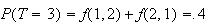 ,
for example. Continuing in this way, we get
,
for example. Continuing in this way, we get
 |
1 |
2 |
3 |
4 |
 |
.1 |
.4 |
.4 |
.1 |
(We are being a little sloppy with our notation by using
" " for
both
" for
both
 and
and
 .
No confusion arises here, but better notation would be to write
.
No confusion arises here, but better notation would be to write
 for
for
 .)
In fact, to find
.)
In fact, to find
 we are simply adding the probabilities for all
 combinations with
 .
This could be written as:
.
This could be written as:
However, if
 ,
then
,
then
 .
To systematically pick out the right combinations of
.
To systematically pick out the right combinations of
 ,
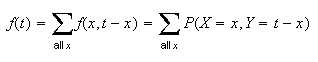
all we really need to do is sum over values of
,
all we really need to do is sum over values of
 and then substitute
 for
for
 .
Then,
.
Then,
So
 would be
(note
 since
since
 can't be 3.)
We can summarize the method of finding the probability function for a function
 of two random variables
 and
and
 as follows:
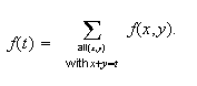
Let
 be the probability function for
 .
Then the probability function for
.
Then the probability function for
 is
is
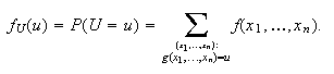
 This can also be extended to functions of three or more r.v.'s
 :
:
 (Note: Do not get confused between the functions
 and
and
 in the above:
 is the joint probability function of the r.v.'s
 whereas
 defines the "new" random variable that is a function of
 and
and
 ,
and whose distribution we want to find.)
,
and whose distribution we want to find.)
This completes the introduction of the basic ideas for multivariate
distributions. As we look at harder problems that involve some algebra, refer
back to these simpler examples if you find the ideas no longer making sense to
you.
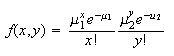
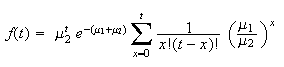
Example: Let
 and
and
 be independent random variables having Poisson distributions with averages
(means) of
be independent random variables having Poisson distributions with averages
(means) of
 and
and
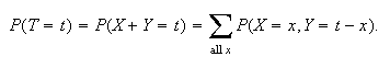
 respectively. Let
 .
Find its probability function,
.
Find its probability function,
 .
.
Solution: We first need to find
 .
Since
.
Since
 and
and
 are independent we know
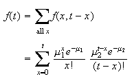
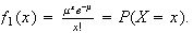
 Using the Poisson probability function,
 where
where
 and
and
 can equal 0, 1, 2,
 .
Now,
.
Now,
 Then
Then
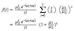
To evaluate this sum, factor out constant terms and try to regroup in some
form which can be evaluated by one of our summation techniques.
If we had a
 on the top inside the
 ,
the sum would be of the form
,
the sum would be of the form
 .
This is the right hand side of the binomial theorem. Multiply top and bottom
by
.
This is the right hand side of the binomial theorem. Multiply top and bottom
by
 to get:
Take a common denominator of
 to get
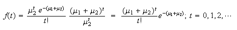
Note that we have just shown that the sum of 2 independent Poisson random
variables also has a Poisson
distribution.
Example: Three sprinters,
 and
and
 ,
compete against each other in 10 independent 100 m. races. The probabilities
of winning any single race are .5 for
,
compete against each other in 10 independent 100 m. races. The probabilities
of winning any single race are .5 for
 ,
.4 for
,
.4 for
 ,
and .1 for
,
and .1 for
 .
Let
.
Let
 and
and
 be the number of races
 and
and
 win.
win.
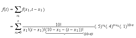
-
Find the joint probability function,

-
Find the marginal probability function,

-
Find the conditional probability function,

-
Are
 and
and
 independent? Why?
-
Let
 .
Find its probability function,
.
Find its probability function,
 .
.
Solution: Before starting, note that
 since there are 10 races in all. We really only have two variables since
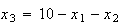 .
However it is convenient to use
.
However it is convenient to use
 to save writing and preserve symmetry.
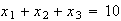
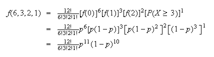
-
The reasoning will be similar to the way we found the binomial distribution in
Chapter 6 except that there are now 3 types of outcome. There are
 different outcomes (i.e. results for races 1 to 10) in which there are
 wins by
 by
by
 ,
and
,
and
 by
by
 .
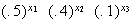
Each of these arrangements has a probability of (.5) multiplied
.
Each of these arrangements has a probability of (.5) multiplied
 times, (.4)
 times, and (.1)
 times in some order;
i.e.,

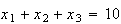
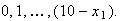
The range for
 is triples
 where each
 is an integer between 0 and 10, and where
 .
.
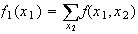
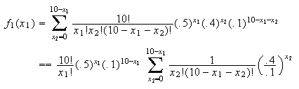
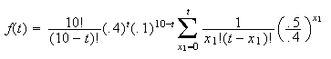
-
It would also be acceptable to drop
 as a variable and write down the probability function for
 only; this is
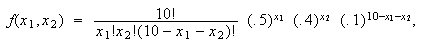 because of the fact that
 must equal
 .
For this probability function
.
For this probability function
 and
and
 .
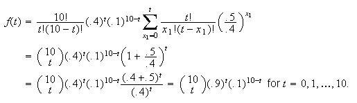
This simplifies finding
.
This simplifies finding
 a little . We now have
 .
The limits of summation need care:
.
The limits of summation need care:
 could be as small as
 ,
but since
,
but since
 ,
we also require
,
we also require
 .
(E.g., if
.
(E.g., if
 then
then
 can win
 ,
or 3 races.) Thus,
,
or 3 races.) Thus,
(Hint: In
 the 2 terms in the denominator add to the term in the numerator, if we ignore
the ! sign.) Multiply top and bottom by
the 2 terms in the denominator add to the term in the numerator, if we ignore
the ! sign.) Multiply top and bottom by
 This
gives
This
gives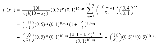
Here
 is defined for
 .
.
Note: While this derivation is included as an example of how
to find marginal distributions by summing a joint probability function, there
is a much simpler method for this problem. Note that each race is either won
by
 (``success'') or it is not won by
 (``failure''). Since the races are independent and
 is now just the number of ``success'' outcomes,
 must have a binomial distribution, with
 and
and
 .
.
Hence
 for
for
 ,
as above.
,
as above.
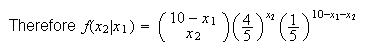
-
Remember that
 ,
so that
,
so that
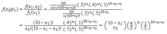 For any given value of
 ranges through
 (So the range of
 depends on the value
 ,
which makes sense: if
,
which makes sense: if
 wins
wins
 races then the most
 can win is
 .)
.)
Note: As in (b), this result can be obtained more simply
by general reasoning. Once we are given that
 wins
wins
 races, the remaining
 races are all won by either
 or
or
 .
For these races,
.
For these races,
 wins
wins
 of the time and
 of the time, because
 and
and
 ;
i.e.,
;
i.e.,
 wins 4 times as often as
 .
More formally
.
More formally
 from the binomial distribution.
-
 and
and
 are clearly not independent since the more races
 wins, the fewer races there are for
 to win. More
formally,
to win. More
formally, (In general, if the range for
 depends on the value of
 ,
then
,
then
 and
and
 cannot be independent.)
-
If
 then
then
The upper limit on
 is
is
 because, for example, if
 then
then
 could not have won more than 7 races. Then
What do we need to multiply by on the top and bottom? Can you spot it before
looking below?
Exercise: Explain to yourself how this answer can be
obtained from the binomial distribution, as we did in the notes following
parts (b) and (c).
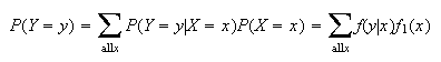
The following problem is
similar to conditional probability problems that we solved in Chapter 4. Now
we are dealing with events defined in terms of random variables. Earlier
results give us things like
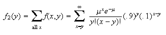
Example: In an auto parts company an average of
 defective parts are produced per shift. The number,
 ,
of defective parts produced has a Poisson distribution. An inspector checks
all parts prior to shipping them, but there is a 10% chance that a defective
part will slip by undetected. Let
,
of defective parts produced has a Poisson distribution. An inspector checks
all parts prior to shipping them, but there is a 10% chance that a defective
part will slip by undetected. Let
 be the number of defective parts the inspector finds on a shift. Find
 .
(The company wants to know how many defective parts are produced, but can only
know the number which were actually detected.)
.
(The company wants to know how many defective parts are produced, but can only
know the number which were actually detected.)
Solution: Think of
 being event
 and
and
 being event
 ;
we want to find
;
we want to find
 .
To do this we'll use
.
To do this we'll use
 We know
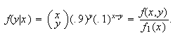
 Also, for a given number
 of defective items produced, the number,
 ,
detected has a binomial distribution with
,
detected has a binomial distribution with
 and
and
 ,
assuming each inspection takes place independently. Then
,
assuming each inspection takes place independently. Then
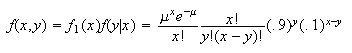
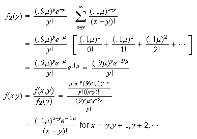
 Therefore
 To get
 we'll need
 .
We have
.
We have
 (
( since the number of defective items produced can't be less than the number
detected.)
since the number of defective items produced can't be less than the number
detected.)
 We could fit this into the summation result
 by writing
 as
as
 .
Then
.
Then
Problems:
-
The joint probability function of
 is:
is:
|
|
 |
 |
0 |
1 |
2 |
|
0 |
.09 |
.06 |
.15 |
 |
1 |
.15 |
.05 |
.20 |
|
2 |
.06 |
.09 |
.15 |
-
Are
 and
and
 independent? Why?
-
Tabulate the conditional probability function,
 .
.
-
Tabulate the probability function of
 .
.
-
In problem 6.14, given that
 sales were made in a 1 hour period, find the probability function for
 ,
the number of calls made in that hour.
,
the number of calls made in that hour.
-
 and
and
 are independent, with
 and
and
 .
Let
.
Let
 .
Find the probability function,
.
Find the probability function,
 .
You may use the result
.
You may use the result
 .
.
Multinomial Distribution
There is only this one multivariate model distribution introduced in this
course, though other multivariate distributions exist. The multinomial
distribution defined below is very important. It is a generalization of the
binomial model to the case where each trial has
 possible outcomes.
Physical Setup: This distribution is the same as binomial
except there are
 types of outcome rather than two. An experiment is repeated independently
 times with
 distinct types of outcome each time. Let the probabilities of these
 types be
 each time. Let
 be the number of times the
 type occurs,
 the number of times the
 occurs,
 ,
,
 the number of times the
 type occurs. Then
 has a multinomial distribution.
Notes:
-
-
 ,
,
If we wish we can drop one of the variables (say the last), and just note that
 equals
 .
.
Illustrations:
-
In the example of Section 8.1 with sprinters A,B, and C running 10 races we
had a multinomial distribution with
 and
and
 .
.
-
Suppose student marks are given in letter grades as A, B, C, D, or F. In a
class of 80 students the number getting A, B, ..., F might have a multinomial
distribution with
 and
and
 .
.
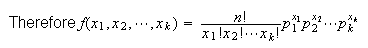
Joint Probability Function: The joint probability function of
 is given by extending the argument in the sprinters example from
 to general
 .
There are
.
There are
 different outcomes of the
 trials in which
 are of the
 type,
type,
 are of the
 type, etc. Each of these arrangements has probability
 since
since
 is multiplied
 times in some order, etc.
 The restriction on the
 's
are
's
are
 and
and
 .
.
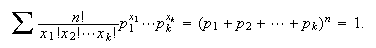
As a check that
 we use the multinomial theorem to get
We have already seen one example of the multinomial distribution in the
sprinter example.
Here is another simple example.
Example: Every person is one of four blood types: A, B, AB
and O. (This is important in determining, for example, who may give a blood
transfusion to a person.) In a large population let the fraction that has type
A, B, AB and O, respectively, be
 .
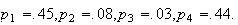
Then, if
.
Then, if
 persons are randomly selected from the population, the numbers
 of types A, B, AB, O have a multinomial distribution with
 (In Caucasian people the values of the
 's
are approximately
's
are approximately
 )
)
Remark: We sometimes use the notation
 to indicate that
 have a multinomial
distribution.
have a multinomial
distribution.
Remark: For some types of problems its helpful to write
formulas in terms of
 and
and
 using the fact that
 In this case we can write the joint p.f. as
 but we must remember then that
 satisfy the condition
 .
.
The multinomial distribution can also arise in combination with other models,
and students often have trouble recognizing it then.
Example: A potter is producing teapots one at a time. Assume
that they are produced independently of each other and with probability
 the pot produced will be "satisfactory"; the rest are sold at a lower price.
The number,
the pot produced will be "satisfactory"; the rest are sold at a lower price.
The number,
 ,
of rejects before producing a satisfactory teapot is recorded. When 12
satisfactory teapots are produced, what is the probability the 12 values of
,
of rejects before producing a satisfactory teapot is recorded. When 12
satisfactory teapots are produced, what is the probability the 12 values of
 will consist of six 0's, three 1's, two 2's and one value which is
 ?
?
Solution: Each time a "satisfactory" pot is produced the
value of
 falls in one of the four categories
 .
Under the assumptions given in this question,
.
Under the assumptions given in this question,
 has a geometric distribution with
 so we can find the probability for each of these categories. We have
 for
for
 and we can obtain
 in various ways:
-
since we have a geometric series.
-
 With some re-arranging, this also gives
 .
.
-
The only way to have
 is to have the first 3 pots produced all being rejects.
 (3 consecutive rejects) =
Reiterating that each time a pot is successfully produced, the value of
 falls in one of 4 categories
 ,
we see that the probability asked for is given by a multinomial distribution,
Mult
,
we see that the probability asked for is given by a multinomial distribution,
Mult :
:
Problems:
-
An insurance company classifies policy holders as class A,B,C, or D. The
probabilities of a randomly selected policy holder being in these categories
are .1, .4, .3 and .2, respectively. Give expressions for the probability that
25 randomly chosen policy holders will include
-
3A's, 11B's, 7C's, and 4D's.
-
3A's and 11B's.
-
3A's and 11B's, given that there are 4D's.
-
Chocolate chip cookies are made from batter containing an average of 0.6 chips
per c.c. Chips are distributed according to the conditions for a Poisson
process. Each cookie uses 12 c.c. of batter. Give expressions for the
probabilities that in a dozen cookies:
-
3 have fewer than 5 chips.
-
3 have fewer than 5 chips and 7 have more than 9.
-
3 have fewer than 5 chips, given that 7 have more than 9.
Markov Chains
Consider a sequence of (discrete) random variables
 each of which takes integer values
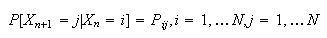
 (called states). We assume that for a certain matrix
 (called the transition probability matrix), the conditional
probabilities are given by corresponding elements of the matrix; i.e.
(called the transition probability matrix), the conditional
probabilities are given by corresponding elements of the matrix; i.e.
 and furthermore that the chain only uses the last state occupied in
determining its future; i.e. that
and furthermore that the chain only uses the last state occupied in
determining its future; i.e. that
 for all
 and
and
 .
Then the sequence of random variables
.
Then the sequence of random variables
 is called a Markov Note_2
Chain. Markov Chain models are the most common simple models for
dependent variables, and are used to predict weather as well as movements of
security prices. They allow the future of the process to depend on the present
state of the process, but the past behaviour can influence the future only
through the present state.
is called a Markov Note_2
Chain. Markov Chain models are the most common simple models for
dependent variables, and are used to predict weather as well as movements of
security prices. They allow the future of the process to depend on the present
state of the process, but the past behaviour can influence the future only
through the present state.
Example. Rain-No rain
Suppose that the probability that tomorrow is rainy given that today is not
raining is
 (and it does not otherwise depend on whether it rained in the past) and the
probability that tomorrow is dry given that today is rainy is
(and it does not otherwise depend on whether it rained in the past) and the
probability that tomorrow is dry given that today is rainy is
 If tomorrow's weather depends on the past only through whether today is wet or
dry, we can define random variables
If tomorrow's weather depends on the past only through whether today is wet or
dry, we can define random variables
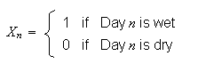 (beginning at some arbitrary time origin, day
 ). Then the random variables
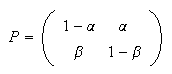
 form a Markov chain with
 possible states and having probability transition matrix
Properties of the Transition Matrix 
Note that
 for all
 and
and
 for all
 This last property holds because given that

 must occupy one of the states

The distribution of 
Suppose that the chain is started by randomly choosing a state for
 with distribution
 .
Then the distribution of
.
Then the distribution of
 is given by
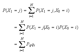 and this is the
 element of the vector
 where
where
 is the column vector of values
 .
To obtain the distribution at time
.
To obtain the distribution at time
 premultiply the transition matrix
 by a vector representing the distribution at time
 Similarly the distribution of
 is the vector
 where
where
 is the product of the matrix
 with itself and the distribution of
 is
is
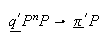
 Under very general conditions, it can be shown that these probabilities
converge because the matrix
Under very general conditions, it can be shown that these probabilities
converge because the matrix
 converges pointwise to a limiting matrix as
 In fact, in many such cases, the limit does not depend on the initial
distribution
In fact, in many such cases, the limit does not depend on the initial
distribution
 because the limiting matrix has all of its rows identical and equal to some
vector of probabilities
because the limiting matrix has all of its rows identical and equal to some
vector of probabilities
 Identifying this vector
 when convergence holds is reasonably easy.
Definition
A limiting distribution of a Markov chain is a vector
( say) of long run probabilities of the individual states so
 Now let us suppose that convergence to this distribution holds for a
particular initial distribution
Now let us suppose that convergence to this distribution holds for a
particular initial distribution
 so we assume that
 Then notice that
 but also
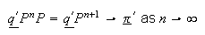 so
so
 must have the property that
 Any limiting distribution must have this property and this makes it easy in
many examples to identify the limiting behaviour of the chain.
Any limiting distribution must have this property and this makes it easy in
many examples to identify the limiting behaviour of the chain.
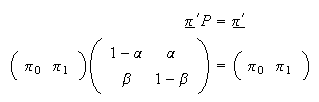
Definition
A stationary distribution of a Markov chain is the column vector
( say) of probabilities of the individual states such that
 .
.
Example: (weather continued)
Let us return to the weather example in which the transition probabilities are
given by the matrix
 What is the long-run proportion of rainy days? To determine this we need to
solve the equations
What is the long-run proportion of rainy days? To determine this we need to
solve the equations
 subject to the conditions that the values
 are both probabilities (non-negative) and add to one. It is easy to see that
the solution
is
are both probabilities (non-negative) and add to one. It is easy to see that
the solution
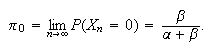
is which is intuitively reasonable in that it says that the long-run probability
of the two states is proportional to the probability of a switch to that state
from the other. So the long-run probability of a dry day is the limit
which is intuitively reasonable in that it says that the long-run probability
of the two states is proportional to the probability of a switch to that state
from the other. So the long-run probability of a dry day is the limit
 You might try verifying this by computing the powers of the matrix
 for
for
 and show that
 approaches the matrix
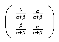 as
as
 There are various mathematical conditions under which the limiting
distribution of a Markov chain unique and independent of the initial state of
the chain but roughly they assert that the chain is such that it forgets the
more and more distant past.
There are various mathematical conditions under which the limiting
distribution of a Markov chain unique and independent of the initial state of
the chain but roughly they assert that the chain is such that it forgets the
more and more distant past.
Example (Gene Model)
TA simple form of inheritance of traits occurs when a trait is governed by a
pair of genes
 and
and
 An
individual may have an
An
individual may have an
 of an
of an
 combination (in which case they are indistinguishable in appearance, or
"
combination (in which case they are indistinguishable in appearance, or
" dominates
 .
Let us call an AA individual dominant,
.
Let us call an AA individual dominant,
 recessive and
 hybrid. When two individuals mate, the offspring
inherits one gene of the pair from each parent, and we assume that these genes
are selected at random. Now let us suppose that two individuals of opposite
sex selected at random mate, and then two of their offspring mate, etc. Here
the state is determined by a pair of individuals, so the states of our process
can be considered to be objects like
hybrid. When two individuals mate, the offspring
inherits one gene of the pair from each parent, and we assume that these genes
are selected at random. Now let us suppose that two individuals of opposite
sex selected at random mate, and then two of their offspring mate, etc. Here
the state is determined by a pair of individuals, so the states of our process
can be considered to be objects like
 indicating that one of the pair is
 and the other is
 (we do not distinguish the order of the pair, or male and female-assuming
these genes do not depend on the sex of the individual)
(we do not distinguish the order of the pair, or male and female-assuming
these genes do not depend on the sex of the individual)
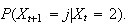
For example, consider the calculation of
 In this case each offspring has probability
 of being a dominant
 ,
and probability of
,
and probability of
 of being a hybrid
(
of being a hybrid
( ).
If two offspring are selected independently from this distribution the
possible pairs are
).
If two offspring are selected independently from this distribution the
possible pairs are
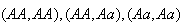 with probabilities
 respectively. So the transitions have probabilities
below:
respectively. So the transitions have probabilities
below: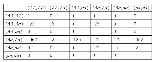
and transition probability
matrix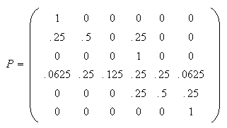
![$\allowbreak$]() What is the long-run behaviour in such a system? For example, the
two-generation transition probabilities are given by
What is the long-run behaviour in such a system? For example, the
two-generation transition probabilities are given by
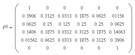 which seems to indicate a drift to one or other of the extreme states 1 or 6.
To confirm the long-run behaviour calculate and :
which seems to indicate a drift to one or other of the extreme states 1 or 6.
To confirm the long-run behaviour calculate and :
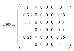 which shows that eventually the chain is absorbed in either of state 1 or
state 6, with the probability of absorption depending on the initial state.
This chain, unlike the ones studied before, has more than one possible
stationary distributions, for example,
which shows that eventually the chain is absorbed in either of state 1 or
state 6, with the probability of absorption depending on the initial state.
This chain, unlike the ones studied before, has more than one possible
stationary distributions, for example,
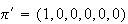 and
and
 and
in these circumstances the chain does not have the same limiting distribution
regardless of the initial state.
and
in these circumstances the chain does not have the same limiting distribution
regardless of the initial state.
Extension of Expectation to Multivariate Distributions
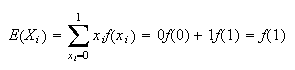
It is easy to extend the definition of expectation to multiple variables.
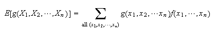
Generalizing
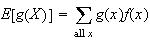 leads to the definition of expected value in the multivariate case
Definition
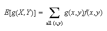 and
and
As before, these represent
the average value of
 and
and
 .
.
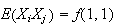
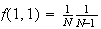
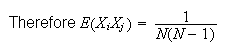
Example: Let the joint probability function,
 ,
be given by
,
be given by
|
|
 |
 |
0 |
1 |
2 |
|
1 |
.1 |
.2 |
.3 |
 |
2 |
.2 |
.1 |
.1 |
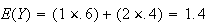
Find
 and
and
 .
.
Solution: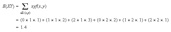
To find
 we have a choice of methods. First, taking
 we
get
we
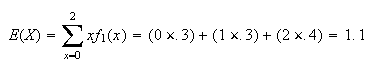
get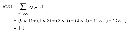 Alternatively, since
 only involves
 ,
we could find
,
we could find
 and use
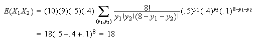
Example: In the example of Section 8.1 with sprinters A, B,
and C we had (using only
 and
and
 in our formulas)
 where A wins
 times and B wins
 times in 10 races. Find
 .
.
Solution: This will be similar to the way
we derived the mean of the binomial distribution but, since this is a
multinomial distribution, we'll be using the multinomial theorem to sum.
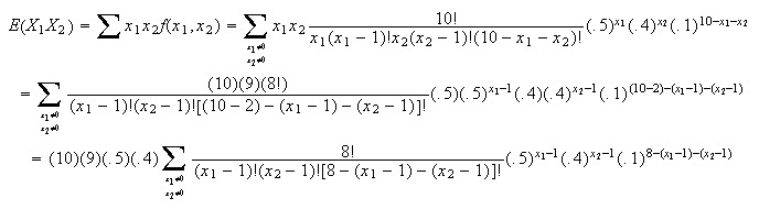 Let
Let
 and
and
 in the sum and we obtain
Property of Multivariate
Expectation: It is easily proved (make sure you can do this) that
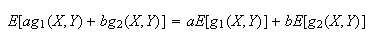 This can be extended beyond 2 functions
 and
and
 ,
and beyond 2 variables
,
and beyond 2 variables
 and
and
 .
.
Relationships between Variables:
Independence is a "yes/no" way of defining a relationship between variables.
We all know that there can be different types of relationships between
variables which are dependent. For example, if
 is your height in inches and
 your height in centimetres the relationship is one-to-one and linear. More
generally, two random variables may be related (non-independent) in a
probabilistic sense. For example, a person's weight
your height in centimetres the relationship is one-to-one and linear. More
generally, two random variables may be related (non-independent) in a
probabilistic sense. For example, a person's weight
 is not an exact linear function of their height
 ,
but
,
but
 and
and
 are nevertheless related. We'll look at two ways of measuring the strength of
the relationship between two random variables. The first is called covariance.
are nevertheless related. We'll look at two ways of measuring the strength of
the relationship between two random variables. The first is called covariance.
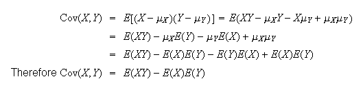
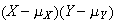
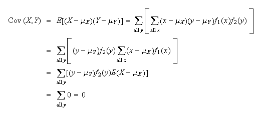
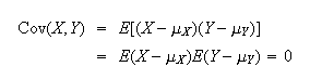
For calculation purposes
this definition is usually harder to use than the formula which follows, which
is proved noting that
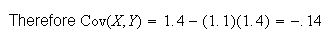
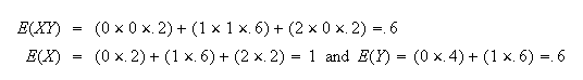
Example:
In the example with joint probability function
 find Cov
 .
.
Solution: We previously calculated
 and
and
 .
Similarly,
.
Similarly,
Exercise: Calculate the covariance of
 and
and
 for the sprinter example. We have already found that
 = 18. The marginal distributions of
 and of
 are models for which we've already derived the mean. If your solution takes
more than a few lines you're missing an easier solution.
are models for which we've already derived the mean. If your solution takes
more than a few lines you're missing an easier solution.
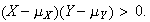
Interpretation of Covariance:
-
Suppose large values of
 tend to occur with large values of
 and small values of
 with small values of
 .
Then
.
Then
 and
and
 will tend to be of the same sign, whether positive or negative. Thus
 will be positive. Hence Cov
 .
For example in Figure bivariatenormal we
see several hundred points plotted. Notice that the majority of the points
are in the two quadrants (lower left and upper right) labelled with "+" so
that for these
.
For example in Figure bivariatenormal we
see several hundred points plotted. Notice that the majority of the points
are in the two quadrants (lower left and upper right) labelled with "+" so
that for these
 A minority of points are in the other two quadrants labelled "-" and for
these
A minority of points are in the other two quadrants labelled "-" and for
these
 .
Moreover the points in the latter two quadrants appear closer to the mean
.
Moreover the points in the latter two quadrants appear closer to the mean
 indicating that on average, over all points generated
 Presumably this implies that over the joint distribution of

 or
or
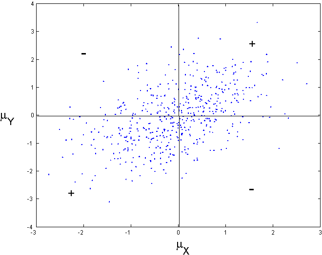
Random points
( with covariance 0.5, variances 1.
|
For example of
 person's
height and
person's
height and
 person's
weight, then these two random variables will have positive covariance.
person's
weight, then these two random variables will have positive covariance.
-
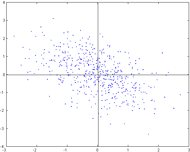
Suppose large values of
 tend to occur with small values of
 and small values of
 with large values of
 .
Then
.
Then
 and
and
 will tend to be of opposite signs. Thus
 tends to be negative. Hence Cov
 .
For example see Figure bivariatenormal2
.
For example see Figure bivariatenormal2
|
Covariance=-0.5,
variances=1
|
For example if
 thickness
of attic insulation in a house and
thickness
of attic insulation in a house and
 heating
cost for the house, then
heating
cost for the house, then
Proof: Recall
 .
Let
.
Let
 and
and
 be independent.
Then
 .
.
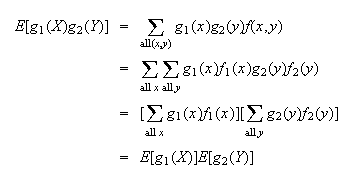
The following theorem gives a direct proof the result above, and is useful in
many other situations.
Proof: Since
 and
and
 are independent,
 .
Thus
.
Thus
 \framebox[0.10in]{}
To prove result (3) above, we just note that if
 and
and
 are independent then
Caution: This result is not reversible. If Cov
 we can not conclude that
 and
and
 are independent. For example suppose that the random variable
 is uniformly distributed on the values
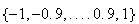 and define
 and
and
 It is easy to see that
Cov
It is easy to see that
Cov but the two random variables
 are clearly related because the points
 are always on a circle.
Example: Let
 have the joint probability function
 ;
i.e.
;
i.e.
 only takes 3 values.
 |
0 |
1 |
2 |
 |
.2 |
.6 |
.2 |
and
 |
0 |
1 |
 |
.4 |
.6 |
are marginal probability functions. Since
 therefore,
 and
and
 are not independent. However,
 So
So
 and
and
 have covariance 0 but are not independent. If Cov
 we say that
 and
and
 are uncorrelated, because of the definition of correlation
Note_3 given below.
are uncorrelated, because of the definition of correlation
Note_3 given below.
-
The actual numerical value of Cov
 has no interpretation, so covariance is of limited use in measuring
relationships.
has no interpretation, so covariance is of limited use in measuring
relationships.
Exercise:
-
Look back at the example in which
 was tabulated and Cov
 .
Considering how covariance is interpreted, does it make sense that Cov
.
Considering how covariance is interpreted, does it make sense that Cov
 would be negative?
-
Without looking at the actual covariance for the sprinter exercise, would you
expect Cov
 to be positive or negative? (If A wins more of the 10 races, will B win more
races or fewer races?)
to be positive or negative? (If A wins more of the 10 races, will B win more
races or fewer races?)
We now consider a second, related way to measure the strength of relationship
between
 and
and
 .
.
The correlation coefficient measures the strength of the linear relationship
between
 and
and
 and is simply a rescaled version of the covariance, scaled to lie in the
interval
and is simply a rescaled version of the covariance, scaled to lie in the
interval
![$[-1,1].$](graphics/noteschap8__736.png) You can attempt to guess the correlation between two variables based on a
scatter diagram of values of these variables at the web
page
You can attempt to guess the correlation between two variables based on a
scatter diagram of values of these variables at the web
page
http://statweb.calpoly.edu/chance/applets/guesscorrelation/GuessCorrelation.html
For
example in Figure guesscorrelation I
guessed a correlation of -0.9 whereas the true correlation coefficient
generating these data was

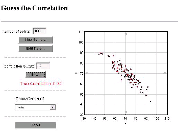
|
Guessing the correlation
based on a scatter diagram of points
|
Properties of
 :
:
-
Since
 and
and
 ,
the standard deviations of
,
the standard deviations of
 and
and
 ,
are both positive,
,
are both positive,
 will have the same sign as Cov
 .
Hence the interpretation of the sign of
.
Hence the interpretation of the sign of
 is the same as for Cov
 ,
and
,
and
 if
if
 and
and
 are independent. When
 we say that
 and
and
 are uncorrelated.
-
 and as
 the relation between
 and
and
 becomes one-to-one and linear.
Proof: Define a new random variable
 ,
where
,
where
 is some real number. We'll show that the fact that
Var
is some real number. We'll show that the fact that
Var leads to 2) above. We
have
leads to 2) above. We
have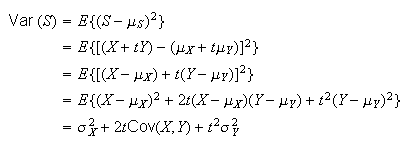
Since
 for any real number
 this quadratic equation must have at most one real root (value of
 for which it is zero). Therefore
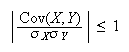
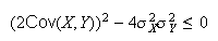 leading to the inequality
 To see that
 corresponds to a one-to-one linear relationship between
 and
and
 ,
note that
,
note that
 corresponds to a zero discriminant in the quadratic equation. This means that
there exists one real number
corresponds to a zero discriminant in the quadratic equation. This means that
there exists one real number
 for which
 But for
Var
But for
Var to be zero,
 must equal a constant
 .
Thus
.
Thus
 and
and
 satisfy a linear relationship.
Exercise: Calculate
 for the sprinter example. Does your answer make sense? (You should already
have found Cov
for the sprinter example. Does your answer make sense? (You should already
have found Cov
 in a previous exercise, so little additional work is
needed.)
in a previous exercise, so little additional work is
needed.)
Problems:
-
The joint probability function of
 is:
is:
|
|
 |
 |
0 |
1 |
2 |
|
0 |
.06 |
.15 |
.09 |
 |
|
|
|
|
|
1 |
.14 |
.35 |
.21 |
Calculate the correlation coefficient,
 .
What does it indicate about the relationship between
.
What does it indicate about the relationship between
 and
and
 ?
?
-
Suppose that
 and
and
 are random variables with joint probability function:
|
|
 |
|
 |
2 |
4 |
6 |
|
-1 |
1/8 |
1/4 |
 |
 |
|
|
|
|
|
1 |
1/4 |
1/8 |
 |
-
For what value of
 are
are
 and
and
 uncorrelated?
-
Show that there is no value of
 for which
 and
and
 are independent.
Mean and Variance of a Linear Combination of Random Variables
Many problems require us to consider linear combinations of random variables;
examples will be given below and in Chapter 9. Although writing down the
formulas is somewhat tedious, we give here some important results about their
means and variances.
Results for Means:
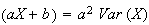
-
 ,
when
,
when
 and
and
 are constants. (This follows from the definition of expectation.) In
particular,
are constants. (This follows from the definition of expectation.) In
particular,
 and
and
 .
.
-
Let
 be constants (real numbers) and
 .
Then
.
Then
 .
In particular,
.
In particular,
 .
.
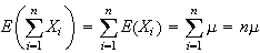
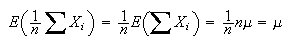
-
Let
 be random variables which have mean
 .
(You can imagine these being some sample results from an experiment such as
recording the number of occupants in cars travelling over a toll bridge.) The
sample mean is
.
(You can imagine these being some sample results from an experiment such as
recording the number of occupants in cars travelling over a toll bridge.) The
sample mean is
 .
Then
.
Then
 .
.
Proof: From (2),
 .
Thus
.
Thus
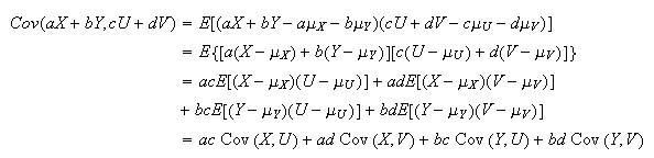
Results for Covariance:
-
Cov

-
Cov
 where
where
 and
and
 are constants.
Proof:
 This type of result can be generalized, but gets messy to write
out.
This type of result can be generalized, but gets messy to write
out.
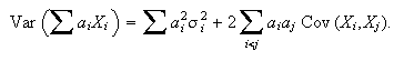
Results for Variance:

Proof: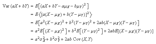
Exercise: Try to prove this result by writing
 as Cov
 and using properties of covariance.
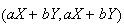
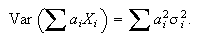
-
Let
 and
and
 be independent. Since Cov
 ,
result 1. gives
,
result 1. gives
 i.e., for independent variables, the variance of a sum
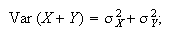
is the sum of the variances. Also note
i.e., for independent variables, the variance of a sum
is the sum of the variances. Also note
 i.e., for independent variables, the variance of a difference is the
sum of the variances.
i.e., for independent variables, the variance of a difference is the
sum of the variances.
-
Let
 be constants and Var
 .
Then
.
Then
 This is a generalization of result 1. and can be proved using either of the
methods used for 1.
This is a generalization of result 1. and can be proved using either of the
methods used for 1.
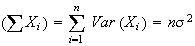
-
Special cases of result 3. are:
-
If
 are independent then Cov
 ,
so that
,
so that
-
If
 are independent and all have the same variance
 ,
then
,
then
Proof of 4 (b):
 .
From 4(a), Var
.
From 4(a), Var
 .
Using Var
.
Using Var
 ,
we get:
,
we get:

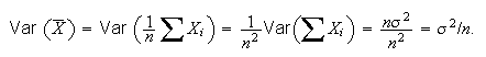
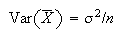
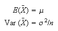
Remark: This result is a very important one in probability
and statistics. To recap, it says that if
 are independent r.v.'s with the same mean
 and some variance
 ,
then the sample mean
,
then the sample mean
 has
has
 This shows that the average
 of
of
 random variables with the same distribution is less variable than any single
observation
random variables with the same distribution is less variable than any single
observation
 ,
and that the larger
,
and that the larger
 is the less variability there is. This explains mathematically why, for
example, that if we want to estimate the unknown mean height
is the less variability there is. This explains mathematically why, for
example, that if we want to estimate the unknown mean height
 in a population of people, we are better to take the average height for a
random sample of
in a population of people, we are better to take the average height for a
random sample of
 persons than to just take the height of one randomly selected person. A sample
of
persons than to just take the height of one randomly selected person. A sample
of
 persons would be better still. There are interesting applets at the url
http://users.ece.gatech.edu/users/gtz/java/samplemean/notes.html
and
http://www.ds.unifi.it/VL/VL_EN/applets/BinomialCoinExperiment.html which
allows one to sample and explore the rate at which the sample mean approaches
the expected value. In Chapter 9 we will see how to decide how large a sample
we should take for a certain degree of precision. Also note that as
persons would be better still. There are interesting applets at the url
http://users.ece.gatech.edu/users/gtz/java/samplemean/notes.html
and
http://www.ds.unifi.it/VL/VL_EN/applets/BinomialCoinExperiment.html which
allows one to sample and explore the rate at which the sample mean approaches
the expected value. In Chapter 9 we will see how to decide how large a sample
we should take for a certain degree of precision. Also note that as
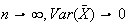 ,
which means that
,
which means that
 becomes arbitrarily close to
 .
This is sometimes called the "law of averages". There is a formal theorem
which supports the claim that for large sample sizes, sample means approach
the expected value, called the "law of large numbers".
.
This is sometimes called the "law of averages". There is a formal theorem
which supports the claim that for large sample sizes, sample means approach
the expected value, called the "law of large numbers".
Indicator Variables
The results for linear combinations of random variables provide a way of
breaking up more complicated problems, involving mean and variance, into
simpler pieces using indicator variables; an indicator variable is just a
binary variable (0 or 1) that indicates whether or not some event occurs.
We'll illustrate this important method with 3
examples.
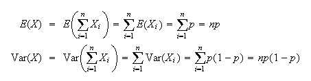
Example: Mean and Variance of a Binomial R.V.
Let
 in a binomial process. Define new variables
 by:
by:
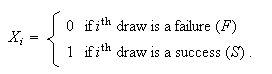
 |
= |
0 if the
 trial was a failure
 |
 |
= |
1 if the
 trial was a success.
 |
i.e.
 indicates whether the outcome "success" occurred on the
 trial. The trick we use is that the total number of successes,
 ,
is the sum of the
,
is the sum of the
 's:
's:

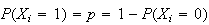
We can find the mean and variance of
 and then use our results for the mean and variance of a sum to get the mean
and variance of
and then use our results for the mean and variance of a sum to get the mean
and variance of
 .
First,
.
First,
 But
But
 since the probability of success is
 on each trial.
 .
Since
.
Since
 or 1,
or 1,
 ,
and therefore
,
and therefore
 Thus
Thus
In the binomial distribution the trials are independent so the
 's
are also independent. Thus
's
are also independent. Thus
These, of course, are the same as we derived previously for the mean and
variance of the binomial distribution. Note how simple the derivation here
is!
Remark: If
 is a binary random variable with
 then
then
 and
Var
and
Var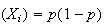 ,
as shown above. (Note that
,
as shown above. (Note that
 is actually a binomial r.v.) In some problems the
 's
are not independent, and then we also need covariances.
's
are not independent, and then we also need covariances.
Example: Let
 have a hypergeometric distribution. Find the mean and variance of
 .
.
Solution: As above, let us think of the setting, which
involves drawing
 items at random from a total of
 ,
of which
,
of which
 are
"
are
" " and
" and
 are
"
are
" items. Define
Then
 as for the binomial example, but now the
 's
are dependent. (For example, what we get on the first draw affects the
probabilities of
's
are dependent. (For example, what we get on the first draw affects the
probabilities of
 and
and
 for the second draw, and so on.) Therefore we need to find
Cov
for the second draw, and so on.) Therefore we need to find
Cov for
for
 as well as
 and
Var
and
Var in order to use our formula for the variance of a sum.
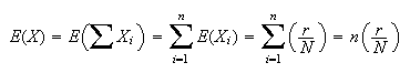
We see first that
 for each of
 .
(If the draws are random then the probability an
.
(If the draws are random then the probability an
 occurs in draw
 is just equal to the probability position
 is an
is an
 when we arrange

 's
and
's
and

 's
in a row.) This immediately gives
's
in a row.) This immediately gives
 since
since
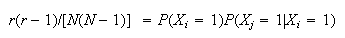
 The covariance of
 and
and
 is equal to
 ,
so we need
,
so we need
 The probability of an
 on both draws
 and
and
 is just
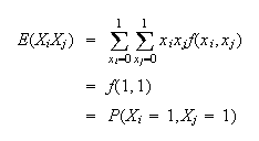
 Thus,
Thus,
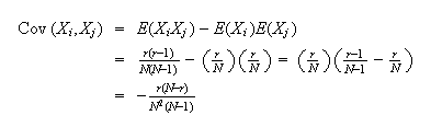 (Does it make sense that Cov
 is negative? If you draw a success in draw
 ,
are you more or less likely to have a success on draw
,
are you more or less likely to have a success on draw
 ?)
Now we find
?)
Now we find
 and
Var
and
Var .
First,
.
First,
 Before finding Var
 ,
how many combinations
,
how many combinations
 are there for which
 ?
Each
?
Each
 and
and
 takes values from
 so there are
 different combinations of
 values. Each of these can only be written in 1 way to make
 .
.
 There are
 combinations with
 (e.g. if
 and
and
 ,
the combinations with
,
the combinations with
 are (1,2) (1,3) and (2,3). So there are
 different combinations.)
Now we can find
In the last two examples, we know
 ,
and could have found
,
and could have found
 and
Var
and
Var without using indicator variables. In the next example
 is not known and is hard to find, but we can still use indicator variables for
obtaining
is not known and is hard to find, but we can still use indicator variables for
obtaining
 and
and
 .
The following example is a famous problem in probability.
.
The following example is a famous problem in probability.
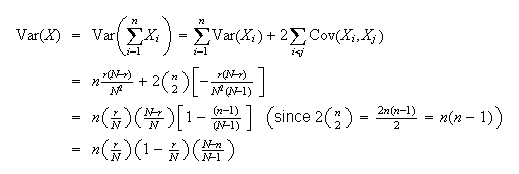
Example: We have
 letters to
 different people, and
 envelopes addressed to those
 people. One letter is put in each envelope at random. Find the mean and
variance of the number of letters placed in the right envelope.
people. One letter is put in each envelope at random. Find the mean and
variance of the number of letters placed in the right envelope.
Solution:
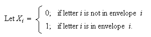 Then
Then
 is the number of correctly placed letters. Once again, the
 's
are dependent (Why?).
's
are dependent (Why?).
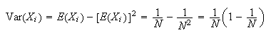
First
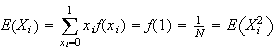 (since there is 1 chance in
 that letter
 will be put in envelope
 )
and then,
)
and then,
Exercise: Before calculating cov
 ,
what sign do you expect it to have? (If letter
,
what sign do you expect it to have? (If letter
 is correctly placed does that make it more or less likely that letter
 will be placed correctly?)
Next,
 (As in the last example, this is the only non-zero term in the sum.) Now,
 since once letter
 is correctly placed there is 1 chance in
 of letter
 going in envelope
 .
.
 For the
covariance,
For the
covariance, (Common sense often helps in this course, but we have found no way of being
able to say this result is obvious. On average 1 letter will be correctly
placed and the variance will be 1, regardless of how many letters there are.)
(Common sense often helps in this course, but we have found no way of being
able to say this result is obvious. On average 1 letter will be correctly
placed and the variance will be 1, regardless of how many letters there are.)
Problems:
-
The joint probability function of
 is given by:
 Calculate
 ,
Var
,
Var
 ,
Cov
,
Cov
 and Var
 .
You may use the fact that
.
You may use the fact that
 and Var
 = .21 without verifying these figures.
-
In a row of 25 switches, each is considered to be "on" or "off". The
probability of being on is .6 for each switch, independently of other switch.
Find the mean and variance of the number of unlike pairs among the 24 pairs of
adjacent switches.
-
Suppose Var
 ,
Var
,
Var
 ,
,
 ;
and let
;
and let
 .
Find the standard deviation of
.
Find the standard deviation of
 .
.
-
Let
 be uncorrelated random variables with mean 0 and variance
 .
Let
.
Let
 .
Find Cov
.
Find Cov
 for
for
 and Var
 .
.
-
A plastic fabricating company produces items in strips of 24, with the items
connected by a thin piece of plastic:
Item 1
--Item 2
-- ...
--Item 24
A cutting machine then
cuts the connecting pieces to separate the items, with the 23 cuts made
independently. There is a 10% chance the machine will fail to cut a connecting
piece. Find the mean and standard deviation of the number of the 24 items
which are completely separate after the cuts have been made. (Hint: Let
 if item
 is not completely separate, and
 if item
 is completely separate.)
Multivariate Moment Generating Functions
Suppose we have two possibly dependent random variables
 and we wish to characterize their joint distribution using a moment generating
function. Just as the probability function and the cumulative distribution
function are, in tis case, functions of two arguments, so is the moment
generating function.
and we wish to characterize their joint distribution using a moment generating
function. Just as the probability function and the cumulative distribution
function are, in tis case, functions of two arguments, so is the moment
generating function.
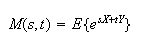
Definition
The joint moment generating function of
 is
is
Recall that if
 happen to be independent,
 and
and
 are any two functions,
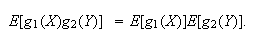 and so with
 and
and
 we obtain, for independent random variables

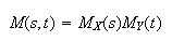 the product of the moment generating functions of
 and
and
 respectively.
There is another labour-saving property of moment generating functions for
independent random variables. Suppose
 are independent random variables with moment generating functions
 and
and
 .
Suppose you wish the moment generating function of the sum
.
Suppose you wish the moment generating function of the sum
 One could attack this problem by first determining the probability function of

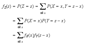 and then calculating
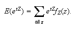 Evidently lots of work! On the other hand recycling
(Eg1g2) with
Evidently lots of work! On the other hand recycling
(Eg1g2) with
 gives
gives
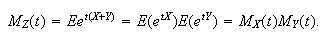
Theorem
The moment generating function of the sum of independent
random variables is the product of the individual moment generating
functions.
For example if both

 and
and
 are independent with the same (Bernoulli) distribution
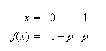 then both have moment generating function
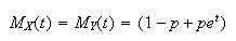 and so the moment generating function of the sum
 is
is
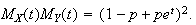 Similarly if we add another independent Bernoulli the moment generating
function is
Similarly if we add another independent Bernoulli the moment generating
function is
 and in general the sum of
 independent Bernoulli random variables is
 the moment generating function of a
Binomial
the moment generating function of a
Binomial distribution. This confirms that the sum of independent Bernoulli random
variables has a
Binomial
distribution. This confirms that the sum of independent Bernoulli random
variables has a
Binomial distribution.
Problems on Chapter 8
-
The joint probability function of
 is given by:
|
|
 |
 |
0 |
1 |
2 |
|
0 |
.15 |
.1 |
.05 |
 |
|
|
|
|
|
1 |
.35 |
.2 |
.15 |
-
Are
 and
and
 independent? Why?
-
Find
 and
and
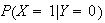
-
For a person whose car insurance and house insurance are with the same
company, let
 and
and
 represent the number of claims on the car and house policies, respectively, in
a given year. Suppose that for a certain group of individuals,
represent the number of claims on the car and house policies, respectively, in
a given year. Suppose that for a certain group of individuals,
 Poisson (mean
 )
and
)
and
 Poisson (mean
 ).
).
-
Consider Problem 2.7 for Chapter 2, which concerned machine recognition of
handwritten digits. Recall that
 was the probability that the number actually written was
 ,
and the number identified by the machine was
,
and the number identified by the machine was
 .
.
-
Are the random variables
 and
and
 independent? Why?
-
What is
 ,
that is, the probability that a random number is correctly identified?
,
that is, the probability that a random number is correctly identified?
-
What is the probability that the number 5 is incorrectly identified?
-
Blood donors arrive at a clinic and are classified as type A, type O, or other
types. Donors' blood types are independent with
 (type A) =
 ,
,
 (type O) =
 ,
and
,
and
 (other type) =
 .
Consider the number,
.
Consider the number,
 ,
of type A and the number,
,
of type A and the number,
 ,
of type O donors arriving before the
,
of type O donors arriving before the
 other type.
-
Find the joint probability function,

-
Find the conditional probability function,
 .
.
-
Slot machine payouts. Suppose that in a slot machine there are
 possible outcomes
 for a single play. A single play costs $1. If outcome
 occurs, you win
 ,
for
,
for
 .
If outcome
.
If outcome
 occurs, you win nothing. In other words, if outcome
 occurs your net profit is
 ;
if
;
if
 occurs your net profit is - 1.
-
Bacteria are distributed through river water according to a Poisson process
with an average of 5 per 100 c.c. of water. What is the probability five 50
c.c. samples of water have 1 with no bacteria, 2 with one bacterium, and 2
with two or more?
-
A box contains 5 yellow and 3 red balls, from which 4 balls are drawn at
random without replacement. Let
 be the number of yellow balls on the first two draws and
 the number of yellow balls on all 4 draws.
-
Find the joint probability function,
 .
.
-
Are
 and
and
 independent? Justify your answer.
-
In a quality control inspection items are classified as having a minor defect,
a major defect, or as being acceptable. A carton of 10 items contains 2 with
minor defects, 1 with a major defect, and 7 acceptable. Three items are chosen
at random without replacement. Let
 be the number selected with minor defects and
 be the number with major defects.
-
Find the joint probability function of
 and
and
 .
.
-
Find the marginal probability functions of
 and of
 .
.
-
Evaluate numerically
 and
and
 .
.
-
Let
 and
and
 be discrete random variables with joint probability function
 for
for
 and
and
 ,
where
,
where
 is a positive constant.
-
Derive the marginal probability function of
 .
.
-
Evaluate
 .
.
-
Are
 and
and
 independent? Explain.
-
Derive the probability function of
 .
.
-
"Thinning" a Poisson process. Suppose that events are
produced according to a Poisson process with an average of
 events per minute. Each event has a probability
 of being a "Type A" event, independent of other events.
-
Let the random variable
 represent the number of Type A events that occur in a one-minute period. Prove
that
represent the number of Type A events that occur in a one-minute period. Prove
that
 has a Poisson distribution with mean
 .
(Hint: let
.
(Hint: let
 be the total number of events in a 1 minute period and consider the formula
just before the last example in Section 8.1).
be the total number of events in a 1 minute period and consider the formula
just before the last example in Section 8.1).
-
Lighting strikes in a large forest region occur over the summer according to a
Poisson process with
 strikes per day. Each strike has probability .05 of starting a fire. Find the
probability that there are at least 5 fires over a 30 day period.
strikes per day. Each strike has probability .05 of starting a fire. Find the
probability that there are at least 5 fires over a 30 day period.
-
In a breeding experiment involving horses the offspring are of four genetic
types with probabilities:
| Type |
1 |
2 |
3 |
4 |
| Probability |
3/16 |
5/16 |
5/16 |
3/16 |
A group of 40 independent offspring are observed. Give expressions for the
following probabilities:
-
There are 10 of each type.
-
The total number of types 1 and 2 is 16.
-
There are exactly 10 of type 1, given that the total number of types 1 and 2
is 16.
-
In a particular city, let the random variable
 represent the number of children in a randomly selected household, and let
 represent the number of female children. Assume that the probability a child
is female is
represent the number of female children. Assume that the probability a child
is female is
 ,
regardless of what size household they live in, and that the marginal
distribution of
,
regardless of what size household they live in, and that the marginal
distribution of
 is as follows:
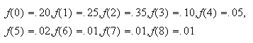
-
In a particular city, the probability a call to a fire department concerns
various situations is as given below:
| 1. fire in a detached home |
-
 |
| 2. fire in a semi detached home |
-
 |
| 3. fire in an apartment or multiple unit residence |
-
 |
| 4. fire in a non-residential building |
-
 |
| 5. non-fire-related emergency |
-
 |
| 6. false alarm |
-
 |
In a set of 10 calls, let
 represent the numbers of calls of each of types
 .
.
-
Give the joint probability function for
 .
.
-
What is the probability there is at least one apartment fire, given that there
are 4 fire-related calls?
-
If the average costs of calls of types
 are (in $100 units) 5, 5, 7, 20, 4, 2 respectively, what is the expected total
cost of the 10 calls?
are (in $100 units) 5, 5, 7, 20, 4, 2 respectively, what is the expected total
cost of the 10 calls?
-
Suppose
 have joint p.f.
 .
If
.
If
 is a function such that for all
 in the range of
 ,
,
then show that
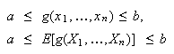
-
Let
 and
and
 be random variables with Var
 ,
Var
,
Var and
and
 .
Find
Var
.
Find
Var .
.
-
Let
 and
and
 have a trinomial distribution with joint probability function
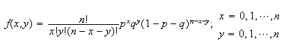 and
and
 .
Let
.
Let
 .
.
-
What distribution does
 have? Either explain why or derive this result.
-
For the distribution in (a), what is
 and
Var
and
Var ?
?
-
Using (b) find
Cov ,
and explain why you expect it to have the sign it does.
,
and explain why you expect it to have the sign it does.
-
Jane and Jack each toss a fair coin twice. Let
 be the number of heads Jane obtains and
 the number of heads Jack obtains. Define
 and
and
 .
.
-
Find the means and variances of
 and
and
 .
.
-
Find Cov

-
Are
 and
and
 independent? Why?
-
A multiple choice exam has 100 questions, each with 5 possible answers. One
mark is awarded for a correct answer and 1/4 mark is deducted for an incorrect
answer. A particular student has probability
 of knowing the correct answer to the
 question, independently of other questions.
-
Suppose that on a question where the student does not know the answer, he or
she guesses randomly. Show that his or her total mark has mean
 and variance
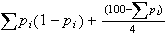 .
.
-
Show that the total mark for a student who refrains from guessing also has
mean
 ,
but with variance
,
but with variance
 .
Compare the variances when all
.
Compare the variances when all
 's
equal (i) .9, (ii) .5.
's
equal (i) .9, (ii) .5.
-
Let
 and
and
 be independent random variables with
 ,
Var
,
Var and Var
 .
Find
Cov
.
Find
Cov .
.
-
An automobile driveshaft is assembled by placing parts A, B and C end to end
in a straight line. The standard deviation in the lengths of parts A, B and C
are 0.6, 0.8, and 0.7 respectively.
-
Find the standard deviation of the length of the assembled driveshaft.
-
What percent reduction would there be in the standard deviation of the
assembled driveshaft if the standard deviation of the length of part B were
cut in half?
-
The inhabitants of the beautiful and ancient canal city of Pentapolis live on
5 islands separated from each other by water. Bridges cross from one island to
another as shown.
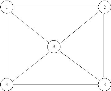
On any day, a bridge can be closed, with probability
 ,
for restoration work. Assuming that the 8 bridges are closed independently,
find the mean and variance of the number of islands which are completely cut
off because of restoration work.
,
for restoration work. Assuming that the 8 bridges are closed independently,
find the mean and variance of the number of islands which are completely cut
off because of restoration work.
-
A Markov chain has a doubly stochastic transition matrix if both the
row sums and the column sums of the transition matrix
 are all
 .
Show that for such a Markov chain, the uniform distribution on
.
Show that for such a Markov chain, the uniform distribution on
 is a stationary distribution.
-
A salesman sells in three cities A,B, and C. He never sells in the same city
on successive weeks. If he sells in city A, then the next week he always
sells in B. However if he sells in either A or B, then the next week he is
twice as likely to sell in city A as in the other city. What is the long-run
proportion of time he spends in each of the three cities?
-
Find
 where
where
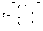
-
Suppose
 and
and
 are independent having Poisson distributions with parameters
 and
and
 respectively. Use moment generating functions to identify the distribution of
the sum
respectively. Use moment generating functions to identify the distribution of
the sum

-
Waterloo in January is blessed by many things, but not by good weather. There
are never two nice days in a row. If there is a nice day, we are just as
likely to have snow as rain the next day. If we have snow or rain, there is an
even chance of having the same the next day. If there is change from snow or
rain, only half of the time is this a change to a nice day. Taking as states
the kinds of weather R, N, and S. the transition probabilities
 are as
follows
are as
follows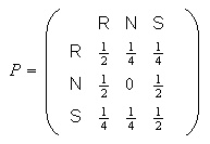 If today is raining, find the probability of Rain, Nice, Snow three days from
now. Find the probabilities of the three states in five days, given (1) today
is raining (ii) today is nice (iii) today is snowing.
If today is raining, find the probability of Rain, Nice, Snow three days from
now. Find the probabilities of the three states in five days, given (1) today
is raining (ii) today is nice (iii) today is snowing.
-
(One-card Poker) A card game, which, for the purposes of this
question we will call Metzler Poker, is played as follows. Each of 2 players
bets an initial $1 and is dealt a card from a deck of 13 cards numbered 1-13.
Upon looking at their card, each player then decides (unaware of the other's
decision) whether or not to increase their bet by $5 (to a total stake of
$6). If both increase the stake ("raise"), then the player with the higher
card wins both stakes-i.e. they get their money back as well as the other
player's $6. If one person increases and the other does not, then the player
who increases automatically wins the pot (i.e. money back+$1). If neither
person increases the stake, then it is considered a draw-each player receives
their own $1 back. Suppose that Player A and B have similar strategies, based
on threshold numbers {a,b} they have chosen between 1
and 13. A chooses to raise whenever their card is greater than or equal to
a and B whenever B's card is greater than or equal
to b.
-
Suppose B always raises (so that b=1). What is the
expected value of A's win or loss for the different possible values of
a=1,2,...,13.
-
Suppose a and b are arbitrary.
Given that both players raise, what is the probability that A wins? What is
the expected value of A's win or loss?
-
Suppose you know that b=11. Find your expected win or
loss for various values of a and determine the
optimal value. How much do you expect to make or lose per game under this
optimal strategy?
-
(Searching a database) Suppose that we are given
3 records,
 initially stored in that order. The cost of accessing the
j'th record in the list is j
so we would like the more frequently accessed records near the front of the
list. Whenever a request for record j is processed,
the "move-to-front" heuristic stores
initially stored in that order. The cost of accessing the
j'th record in the list is j
so we would like the more frequently accessed records near the front of the
list. Whenever a request for record j is processed,
the "move-to-front" heuristic stores
 at the front of the list and the others in the original order. For example if
the first request is for record
at the front of the list and the others in the original order. For example if
the first request is for record
 then the records will be re-stored in the order
 Assume that on each request, record
 is requested with probability
 for
for

-
Show that if
 the
permutation that obtains after
the
permutation that obtains after
 requests for records (e.g.
 ),
then
),
then
 is a Markov chain.
-
Find the stationary distribution of this Markov chain. (Hint: what is the
probability that
 takes the form
 ?).
?).
-
Find the expected long-run cost per record accessed in the case
 respectively.
-
How does this expected long-run cost compare with keeping the records in
random order, and with keeping them in order of decreasing values of
 (only
possible if we know
(only
possible if we know