3.4 The Hartman-Grobman theorem

We showed in Section 3.1 that if $\ol{x}$ is a nonlinear sink or source, then in a neighbourhood of $\ol{x}$, the nonlinear system

 

x' = f(x) (3.14)

has the same qualitative structure as the linear system

 

y' = Ay, (3.15)

where $A = Df (\ol{x})$. We shall show that this is true if $\ol{x}$ is a hyperbolic equilibrium point. The general result is known as the Hartman-Grobman Theorem.

Let us begin with an example

Example 3.4.1:     Consider the nonlinear system in R²

$$\left\{ \begin{array}{l} x'_{1} = x_{1} (1-x_{1}), \\ x'_{2} = - 2 x_{2} \, . \end{array} \right.$$ (3.16)

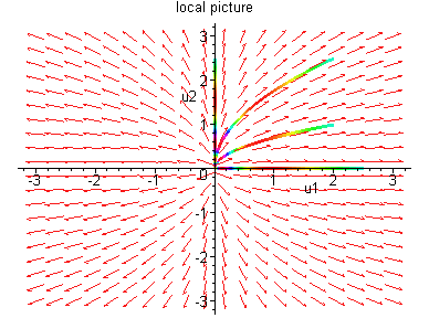
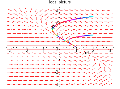
This system has two equilibrium points (0,0) and (1,0). The following are the linearizations of (3.16) at these equilibria and their phase portraits.

          

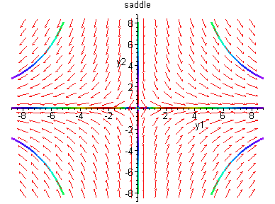
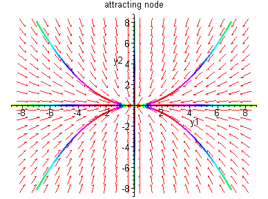
Linearization at (0,0).            Linearization at (1,0).

y' = Df (0,0) y,            y' = Df (1,0) y,

$$Df (0,0) = \left( \begin{array}{lr} 1 & 0 \\ 0 & -2 \end{array} \right).$$            $$Df (1,0) = \left( \begin{array}{rr} -1 & 0 \\ 0 & -2 \end{array} \right).$$

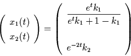
The solution of (3.16) can be solved explicitly as follows

$$\left( \begin{array}{l} x_{1} (t) \\ x_{2} (t) \end{array} \r... ...t} k_{1} + 1-k_{1}}} \\ \\ e^{-2t} k_{2} \end{array} \right)$$

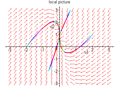
The phase portrait is shown below.

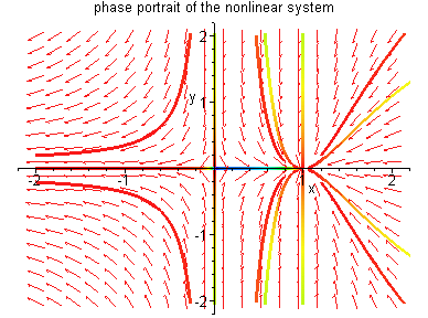
phase portrait of the nonlinear system

Example 3.4.1 Simulation

It is easy to see that the linearizations give a reliable description of the nonlinear orbits near the equilibrium points.

For convenience, we shall assume that the equilibrium point $\ol{x} = 0$. We need the following definition.

Definition 3.4.1:     The systems (3.14) and (3.15) are said to be topologically equivalent in a neighbourhood of the origin if there exists a homeomorphism $h : U \raro V$, where U and V are some open sets containing the origin, which maps trajectories of (3.14) in U onto those of (3.15) in V and preserves the orientation. If, in addition, h preserves the parameterization by time, then (3.14) and (3.15) are said to be topologically conjugate in a neighbourhood of the origin.

Clearly, if two linear systems x' = A₁ x and y' = A₂ y in Rⁿ are linearly equivalent, then they are topologically equivalent. In fact, let k > 0 and P be a nonsingular matrix such that

$$A_{2} = k P^{-1} A_{1} P \, .$$

Setting y = h(x) = P^-1 x, then $y' = P^{-1} x' = P^{-1} A_{1} Py = \frac{1}{k} A_{2} y$.

Let t = sk. Then

$$\frac{dy}{dt} = \frac{dy}{ds} \frac{ds}{dk} = \frac{dy}{ds} \frac{1}{k} \, ,$$

which implies

$$\frac{dy}{ds} = A_{2} y \, .$$

Thus the mapping h, which is clearly a homeomorphism, maps trajectories of x' = A₁ x onto trajectories of y' = A₂ y and preserves the orientation since k > 0. In the case k=1, h preserves the parameterization by time and thus the two linear systems are topologically conjugate.

Theorem 3.4.1: (Hartman-Grobman)     Let $\Omega \subset R^{n}$ be an open set containing the origin, let $f \in C^{1} (\Omega )$, and let $\phi_{t}$ be the flow of the nonlinear system (3.14). Suppose that f(0) = 0 and the matrix A =Df(0) has no eigenvalue with zero real part. Then there exists a homeomorphism $h : U \raro V$, U and V being open sets containing the origin, such that $\forall \; x_{0} \in U$

$$h \circ \phi_{t} (x_{0}) = e^{At} h(x_{0}) \,, \quad t \in J(x_{0}) \, , \quad J(x_{0}) \subset R$$

being an open interval containing zero.

Proof:     See P. Hartman, Ordinary Differential Equations, 2nd Ed., 1973, P. 244-250.

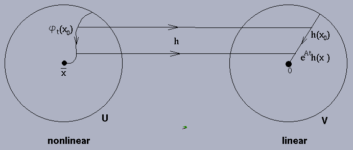
Theorem 3.4.1 tells us that h maps trajectories of (3.14) in a neighbourhood of the equilibrium point onto trajectories of (3.15) in a neighbourhood of the origin and preserves the parameterization, and thus systems (3.14) and (3.15) are topologically conjugate in a neighbourhood of the origin.

Illustration:

Remark:     The above theorem was proved independently by P. Hartman in 1960 and the Russian mathematician D.M. Grobman in 1959.

Example 3.4.2:     Consider the system

$$\left\{ \begin{array}{l} x' = -x, \\ y' = y + x^{2}. \end{array} \right.$$ (3.17)

The solution of (3.17) is given by

$$\phi_{t} (x_{0}, y_{0}) = \left( x_{0} e^{-t}, y_{0} e^{t} + \frac{x_{0}^{2}}{3} (e^{t} - e^{-2t})\right)^{T} \, .$$

The linearization of (3.17) at (0,0) is

$$\left\{ \begin{array}{l} x' = - x, \\ y' = y, \end{array} \right.$$ (3.18)

whose solution is

$$e^{At} \left( \begin{array}{l} x_{0} \\ y_{0} \end{array} \ri... ...ft[ \begin{array}{rl} -1 & 0 \\ 0 & 1 \end{array} \right] \, .$$

Define the homeomorphism h by $h(x,y) = \left( x, y+ \frac{x^{2}}{3} \right)^{T}$.

Then

$$\begin{eqnarray*}h \circ \phi_{t} ( x_{0}, y_{0}) & = & \left( x_{0} e^{-t} , y_... ...{2}}{3} \right) e^{t} \right)^{T} = e^{At} h (x_{0}, y_{0}) \, . \end{eqnarray*}$$

          

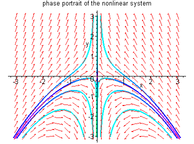
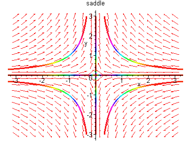
Example 3.4.2 Simulation

Remark:

1.

In the above example, we actually have found a global homeomorphism which maps trajectories of (3.17) onto trajectories of (3.18). But this does not happen very often in general.

2.

The images of the stable and unstable subspaces of (3.18), i.e. x-axis and y-axis, in Example 3.4.2, under the mapping h^-1 are the curves $y = - \frac{1}{3} x^{2}$ and y-axis, respectively, which are invariant sets of (3.17). All solutions of (3.17) starting on the curve $y = - \frac{1}{3} x^{2}$ tend to the origin as $t \raro \infty$. Moreover the curve $y = - \frac{1}{3} x^{2}$ is tangent to the x-axis at the origin.

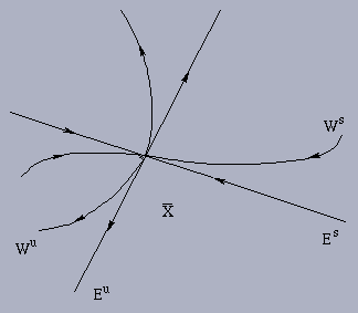
In general, if $\ol{x}$ is a saddle point of the system (3.14) with $f(\ol{x}) = 0$, then the images of the stable subspace E^s and the unstable subspace of the linearized system (3.15), in a neighbourhood of the origin, under the mapping h^-1 are surfaces W^s and W^u, which are called local stable manifold and local unstable manifold of $\ol{x}$ respectively, and can be defined as follows:

$$W^{s} (\ol{x}) = \left\{ x \in U \biggl\vert \phi_{t} (x) \in... ...(x) \raro \ol{x} \quad \mbox{as} \quad t \raro \infty \right\}$$

$$W^{u} (\ol{x}) = \left\{ x \in U \biggl\vert \phi_{t} (x) \in... ...ro \ol{x} \quad \mbox{as} \quad t \raro - \infty \right\} \, .$$

The relations between W^s/W^u and E^s/E^u are given in the next theorem.

Theorem 3.4.2: (Stable/unstable manifold)     Let $\Omega \subset R^{n}$ be an open set containing $\ol{x}$, let $f \in C^{1} (\Omega )$, and let $\phi_{t}$ be the flow of the system (3.14). Suppose that $f(\ol{x}) = 0$ and that $Df(\ol{x})$ has k eigenvalues with negative real parts and n-k eigenvalues with positive real parts. Then there exists k-dimensional stable manifold W^s tangent to E^s at $\ol{x}$, and n-k-dimensional unstable manifold W^u tangent to E^u at $\ol{x}$, such that W^s and W^u are positively invariant and negatively invariant sets of (3.14), respectively, and

$$\begin{array}{lll} \forall \; x_{0} \in W^{s}, & {\dss\lim_{t... ...m_{t \raro -\infty}} \phi_{t} (x_{0}) = \ol{x} \, . \end{array}$$

Proof:     See Perko, Differential Equations/Dynamical Systems, P. 108-111.

Illustration:

Remark:     The stable and unstable manifolds W^s and W^u, in Theorem 3.4.2, are only defined in a small neighbourhood of the equilibrium point $\ol{x}$ and are therefore referred to as local stable and unstable manifolds. We define the global stable and unstable manifolds of (3.14) at $\ol{x}$ by letting points in W^s flow backward in time and those in W^u flow forward in time.

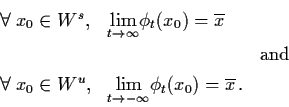
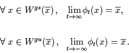
The global stable manifold of (3.14) at $\ol{x}$ is given by

$$W^{gs} (\ol{x}) = \bigcup_{t \leq 0} \phi_{t} W^{s} (\ol{x}) \, .$$

The global unstable manifold of (3.14) at $\ol{x}$ is given by

$$W^{gu} (\ol{x}) = \bigcup_{t \geq 0} \phi_{t} W^{u} (\ol{x}) \, .$$

It can be shown that the global stable and unstable manifolds $W^{gs} (\ol{x})$ and $W^{gu} (\ol{x})$ are unique, invariant and

$$\begin{array}{ll} \forall \; x \in W^{gs} (\ol{x}) \, , & {\d... ...s\lim_{t \raro - \infty}} \phi_{t} (x) = \ol{x} \, .\end{array}$$

It is easy to see that the curve $y = - \frac{1}{3} x^{2}$, in example 3.4.2, is the global stable manifold and the y-axis is the global unstable manifold.

The linearization of a non-linear system can fail to give reliable information about the orbits, if a certain restriction (hyperbolic) does not hold.

Example 3.4.3:     Consider the nonlinear system

$$\left\{ \begin{array}{l} x'_{1} = - x_{1}, \\ x'_{2} = x_{2}^{3}. \end{array} \right.$$

Then $x_{1} = ke^{\frac{1}{2x_{2}^{2}}}$ and the origin is a nonlinear saddle.

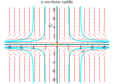Linearization at (0,0) is given by

$$y' = Df (0,0) y \, ,$$

$$\mbox{where} \qquad Df (0,0) = \left( \begin{array}{rl} -1 & 0 \\ 0 & 0 \end{array}\right) .$$

The phase portrait is shown on the right which illustrates that linearization fails to give reliable information.

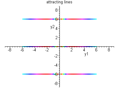
The source of the failure is that the matrix Df(0,0) has a zero eigenvalue.

Example 3.4.3 Simulation

Example 3.4.4:     Consider the nonlinear system

$$\left\{ \begin{array}{l} x'_{1} = - x_{2} - x_{1} (x_{1}^{2} ... ...2} = x_{1} - x_{2} (x_{1}^{2} + x_{2}^{2}), \end{array}\right.$$

which is a nonlinear spiral.

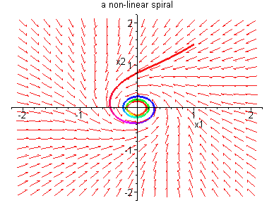
But the linearization at (0,0) is

$$y' = Df (0,0) y \, , \quad Df (0,0) = \left( \begin{array}{lr} 0 & -1 \\ 1 & 0 \end{array} \right) ,$$

which is a centre.

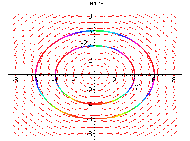
The source of the failure is that the matrix Df(0,0) has eigenvalues with zero real parts.

Finally, to conclude this section, we come back to the population growth model which was considered in Section 3.2.

Example 3.4.4 Simulation

Example 3.4.5:     Consider the nonlinear system

$$\left\{ \begin{array}{l} x' = x - x^{2} - xy, \\ y' = \frac{... ... - \frac{1}{4} y^{2} - \frac{3}{4} xy \, . \end{array} \right.$$

There are four equilibrium points.

1.

(0,0), neither species win and there is natural annihilation;

2.

(1,0), ``A'' wins;

3.

(0,2), ``B'' wins;

4.

$\left( \frac{1}{2}, \frac{1}{2} \right)$, a state of coexistence.

By plotting the phase portrait, we would like to see the initial conditions which, as $t \raro \infty$, would give rise to the above equilibrium states.

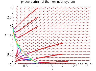
The first step is to characterize the nature of each equilibrium point according to the linearization.

$$A = Df (\ol{x}) = \left[ \begin{array}{cc} 1-2x-y & -x \\ - ... ...rac{3}{4} x \end{array} \right]_{x=\ol{x} \atop y=\ol{y}} \, .$$

Case 1:      $(\ol{x}, \ol{y}) =(0,0)$.

$$A =\left[ \begin{array}{cc} 1 & 0 \\ 0 & \frac{1}{2} \end{array} \right] \, , \lambda_{1} = 1, \lambda_{2} = \frac{1}{2}.$$

Thus (0,0) is a source.

Eigenvectors $u_{1} = {1 \choose 0}$, $u_{2} = {0 \choose 1}$.

Case 2:      $(\ol{x}, \ol{y}) = (1,0)$.

$$A = \left[ \begin{array}{rr} -1 & -1 \\ 0 & - \frac{1}{4} \e... ..., ,& u_{2} = \left( 1, - \frac{3}{4} \right). \end{array} \, .$$

Thus (1,0) is a sink.

Case 3:      $(\ol{x}, \ol{y})=(0,2)$.

$$A = \left[ \begin{array}{rr} -1 & 0 \\ - \frac{3}{2} & - \fr... ...bda_{2} = -\frac{1}{2} & u_{2} = (0,1) \end{array}\right\} \,$$

(0,2) is a sink.

Case 4:      $(\ol{x}, \ol{y}) =\left( \frac{1}{2}, \frac{1}{2} \right)$.

$$A = \left[ \begin{array}{r} - \frac{1}{2} - \frac{1}{2} \\ -... ... \frac{1}{16} \left( -5 - \sqrt{57} \right) < 0. \end{array} .$$

Thus $\left( \frac{1}{2}, \frac{1}{2} \right)$ is a saddle.

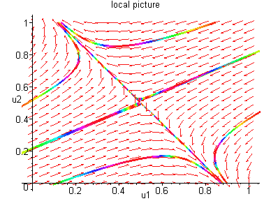
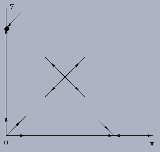
We may ``paste'' these local pictures onto a huge picture of the phase plane as follows:

Explanation:

1)

Equilibrium points A and B, representing ``win'' of one species over another, are sinks, hence they attract nearby solution trajectories. They are said to be stable. (This will be formally defined and discussed in the next section.)

2)

The origin 0 is a source, being unstable - nearby solution trajectories are repelled away, hence there is no possibility that both populations would be eliminated.

3)

The last equilibrium point represents peaceful coexistence, and is a saddle and hence the chances of reaching it are very rare. Only points which lie on the stable manifolds $W^{s}(\ol{x})$ of the equilibrium points will be attracted arbitrarily close to it. On the other hand, virtually all other points $\{ (x,y) \mid x>0, y>0 \}$ will be attracted to either (1,0) or (0,2).

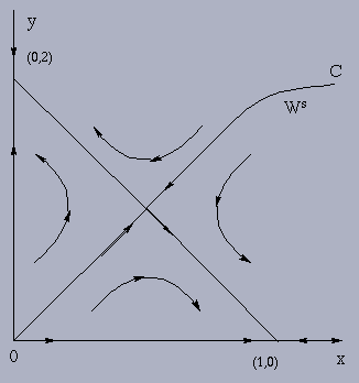
A more complete picture of the phase portrait is shown below.

Example 3.4.5 Simulation

Remark: In applications, coexistence is very important. To have coexistence, one should control the population so that neither species will die out.

The curve C in the diagram, which is, in fact, the stable manifold of the equilibrium point $\left( \frac{1}{2}, \frac{1}{2} \right)$, separates regions of the quadrant which are attracted to the equilibrium points (1,0) and (0,2). These two regions are formally called the basins of attraction of the attractive equilibrium points (1,0) and (0,2) and are usually denoted by

$$\begin{array}{l} W(1,0) = \Bigl\{ (x,y) \in R_{t}^{2} \, \mid... ...(0,2) \quad \mbox{as} \quad t \raro \infty \Bigr\}. \end{array}$$

The determination, or at least estimation, of the basins of attraction of an equilibrium point, is an important aspect of dynamical systems theory and its application. For example, given a reasonable model of a mechanical system, (e.g. bridge, electrical circuits, solar system), which has a stable equilibrium $\ol{x}$, to what points in phase space can we perturb the system and be ensured that the equations of motion of the system will bring it back to that equilibrium point?